Prefill-decode disaggregation: a DistServe and Splitwise paper review

Reading-register key

• From the paper: claims drawn from one of the two source papers’ text, equations, tables, or figures.
• [Analysis]: the publication’s own reasoned assessment, distinct from any claim either paper makes.
• [External comparison]: comparison to named prior or follow-up work outside the two source papers.
• [Reviewer Perspective]: a critical or speculative assessment that goes beyond what either paper proves.

Figure 2 of DistServe (arXiv:2401.09670), reproduced for editorial coverage.

Section 1: Cluster scope

This review covers two systems papers that independently proposed the same architectural shift for large-language-model serving in late 2023 and early 2024: DistServe by Zhong et al. (OSDI 2024) ¹ and Splitwise by Patel et al. (ISCA 2024). ² Both papers argue that the two computational phases of autoregressive LLM inference, prefill, where the prompt is processed in a single parallel pass to produce the first output token, and decode, where subsequent tokens are generated one at a time, should not run on the same GPU pool. They should be disaggregated onto separate machines with phase-specific resource allocation.

The two papers reach the same conclusion from different angles. DistServe frames the problem around service-level objectives, Time-to-First-Token (TTFT) and Time-Per-Output-Token (TPOT), and shows that colocated serving forces a goodput penalty because the two phases interfere with each other on the same batch. ³ Splitwise frames it around hardware utilisation: prefill is compute-bound and benefits from H100-class FLOPs, while decode is memory-bandwidth-bound and runs almost as fast on cheaper A100s. ⁴ Both observations are correct, and both papers’ proposed fix is the same: split the phases across separate machine pools, transfer the KV cache between them, and schedule the two pools independently.

[Analysis] Reading the two papers together rather than separately is the right way to understand what is now the dominant LLM-serving architecture. As of May 2026, prefill-decode disaggregation is shipped in vLLM as an experimental feature, ⁵ is the headline architecture of NVIDIA’s Dynamo serving framework, ⁶ and underlies Moonshot AI’s Kimi inference stack via the Mooncake paper. ⁷ A practitioner deploying LLM serving in production today encounters disaggregation as a real configuration choice; DistServe and Splitwise are the two papers that made the case for it.

Section 2: TL;DR for the cluster

LLM inference has two phases that look nothing like each other. Prefill processes the whole prompt in one big matrix multiplication and is bottlenecked by compute. Decode generates output tokens one at a time, each step a small matrix-vector product bottlenecked by how fast the GPU can read the model weights and the growing key-value cache from memory. When both phases run on the same GPU as part of one continuous batch, the default since vLLM popularised PagedAttention ⁸ , the long prefill stalls the short decodes that share the batch, blowing up tail latency.

DistServe and Splitwise both fix this by moving prefill and decode to separate GPU pools. After a request finishes prefill on a prefill GPU, the per-token KV cache (the model’s attention state for every prompt token) is transferred over a fast interconnect, NVLink within a node, InfiniBand across nodes, to a decode GPU, which then generates tokens autoregressively until the response finishes. Each pool batches and schedules independently, so a long prefill on one machine no longer delays a decode on another. DistServe reports up to 4.48× higher sustainable request rate at the same SLO target versus vLLM colocated on a summarisation workload; ⁹ Splitwise reports 1.4× throughput at 20% lower cost versus a homogeneous H100 baseline at iso-cost. ¹⁰

The trade-off both papers acknowledge: disaggregation adds a KV-cache transfer step and roughly doubles the minimum GPU count for any deployment (you can no longer share one GPU between phases). The gain only beats colocation when the workload’s TTFT and TPOT targets are stringent enough that the interference cost outweighs the transfer cost, broadly, on chat-style workloads with sub-second TTFT SLOs at moderate-to-high request rates.

Section 2.5: Glossary

Term	Plain-English explanation	First appears in
Prefill	The first phase of LLM inference: the model reads the whole prompt in one parallel pass and produces the first output token. Compute-bound.	Section 2
Decode	The second phase: the model generates output tokens one at a time, each step reading the model weights and KV cache from memory. Memory-bandwidth-bound.	Section 2
KV cache	The stored key and value tensors from the attention layers, one entry per prompt-or-generated token. Decode reads it every step; it grows as generation proceeds.	Section 2
TTFT	Time-To-First-Token. Wall-clock latency from request arrival to the first output token leaving the server. Dominated by prefill time.	Section 2
TPOT	Time-Per-Output-Token. The average inter-token latency during generation. Dominated by decode time.	Section 2
ITL	Inter-Token Latency. Used interchangeably with TPOT in vLLM documentation.	Section 7
SLO	Service-Level Objective. A latency target the server is expected to meet for some percentage of requests, e.g. “P90 TTFT < 200ms”.	Section 2
Goodput	Throughput measured only against requests that meet the SLO. A request served too slowly is dropped from the count.	Section 3
Continuous batching	The vLLM-default scheduling pattern: at every step, the next batch can pull in new prefill requests alongside ongoing decodes. The pattern that creates prefill-decode interference.	Section 4
NVLink	NVIDIA’s high-bandwidth (600 GB/s on A100/H100) GPU-to-GPU interconnect inside a single node.	Section 5
InfiniBand	A high-bandwidth network fabric (200-400 Gbps in DGX-class machines) used to connect GPUs across separate nodes.	Section 5
Tensor parallelism (TP)	Splitting individual matrix multiplications across multiple GPUs. Commonly used inside a single node.	Section 5
Pipeline parallelism (PP)	Splitting the model’s layers across multiple GPUs, with activations passed between them. Used across nodes.	Section 5
PagedAttention	The vLLM-introduced technique that stores the KV cache in fixed-size blocks like virtual memory pages, eliminating fragmentation.	Section 4
Continuous-batching baseline	Synonym for vLLM-style colocated serving with continuous batching, used as the comparison anchor in both papers.	Section 9
From the paper: prefix	Content directly supported by one of the two papers’ text, equations, tables, or figures.	Throughout
[Analysis] label	The publication’s own reasoned assessment, distinct from what either paper itself claims.	Throughout
[Reviewer Perspective] label	A critical or speculative assessment that goes beyond what either paper proves.	Section 11 + 12
[External comparison] label	A comparison to prior or follow-up work outside DistServe and Splitwise.	Section 4 + 11

Section 3: Problem formalisation

Notation.

Symbol	Type	Meaning	First appears in
$L$	int	Prompt length in tokens	Section 3
$O$	int	Output length in tokens	Section 3
$b$	int	Batch size at a given scheduler step	Section 3
$h$	int	Hidden dimension of the transformer	Section 6
$m$	int	FFN intermediate dimension	Section 6
$T_{\text{prefill}}$	seconds	Latency of the prefill phase for one request	Section 6
$T_{\text{decode}}$	seconds	Latency of one decode step across the active batch	Section 6
$\text{TTFT}$	seconds	Time-to-first-token, end-to-end	Section 3
$\text{TPOT}$	seconds	Time-per-output-token, averaged across decode steps	Section 3
$\text{SLO}_{\text{TTFT}}, \text{SLO}_{\text{TPOT}}$	seconds	Latency targets the server is expected to meet	Section 3
$\alpha$	fraction in $[0,1]$	SLO attainment goal (e.g., 0.9 for P90)	Section 3
$R$	requests/sec	Sustainable request arrival rate	Section 3
$G$	requests/sec/GPU	Per-GPU goodput	Section 3

Setting. Both papers consider an online LLM-serving cluster of $N$ GPUs running an autoregressive transformer of fixed weights. Requests arrive at rate $R$ with prompt length $L$ and output length $O$ drawn from a workload distribution. The server’s job is to maximise $R$ subject to the joint SLO that at least an $\alpha$ fraction of served requests satisfy both $\text{TTFT} < \text{SLO}_{\text{TTFT}}$ and $\text{TPOT} < \text{SLO}_{\text{TPOT}}$.

Why the problem is hard (the structural argument both papers make). From the paper: a single autoregressive request alternates between one prefill step and $O-1$ decode steps. Prefill takes time proportional to $L$ (or super-linear in $L$ when the attention term dominates); each decode step is roughly constant in the active batch. On a colocated server using continuous batching, the scheduler is free to mix prefill and decode steps in the same micro-batch. From DistServe Figure 2: a single prefill request entering a batch of decodes pushes both the TTFT of that prefill and the TPOT of every ongoing decode in the batch, interference is bidirectional. From DistServe Figure 3: prefill throughput saturates at small batch sizes because compute is the bottleneck, whereas decode throughput scales near-linearly with batch size because the GPU is memory-bound and adding more decodes amortises weight reads.

The structural mismatch: the two phases want different batch sizes, different parallelism strategies, and different hardware properties. Both papers argue the only clean way to give each phase what it wants is to put them on different machines.

Goodput as the optimisation target. DistServe formalises the cost metric as per-GPU goodput $G$: from the paper, “the maximum request rate that can be served adhering to the SLO attainment goal (say, 90%) for each GPU provisioned.” Higher $G$ means lower cost per query. The whole DistServe paper is structured as a search over deployment configurations that maximise $G$ under a workload distribution and SLO pair.

Splitwise’s framing. Splitwise instead casts the problem as a multi-objective optimisation over throughput, cost, and power. From the paper, the prompt phase utilises compute efficiently while the token phase remains memory-bound; this asymmetry means hardware choices that are optimal for one phase are wasteful for the other.

Assumption audit.

• Both papers assume the workload distribution is known. Schedulers in both systems pre-compute deployment plans against a profiled distribution of $L, O$. [Analysis] Production traces drift, Splitwise’s own Figure 3a/3b shows coding versus conversation traces have very different prompt and output length distributions, so the planner must re-run when traffic mix changes. Splitwise addresses this with a dynamic “mixed pool” that absorbs imbalance; DistServe does not.
• Both papers assume the KV-cache transfer can be hidden. DistServe (Figure 10) reports KV-cache transmission is <0.1% of total latency for OPT-175B with NVLink colocation; Splitwise (KV-cache transfer optimisation section) reports 0.8% E2E with layer-wise asynchronous transfer over InfiniBand, down from 64% for naive serialised transfer. [Analysis] Potentially limiting assumption, the hidden cost depends on having InfiniBand or NVLink between the two pools. RoCE-only or PCIe-only deployments will see higher transfer overhead.
• Both papers assume autoregressive transformer decoding. From DistServe limitations: the system targets autoregressive LLM inference only. Speculative decoding, parallel decoding, and non-autoregressive generation change the phase boundaries.

Section 4: Motivation and gap

The real-world problem. Production LLM serving in 2024 was dominated by continuous-batching systems, vLLM, TGI, TensorRT-LLM, that mixed prefill and decode steps in the same batch. ⁵ The architecture is throughput-optimal in isolation but creates two operational pathologies.

Pathology 1, TTFT spikes under load. When the scheduler decides to attach a long-prompt prefill to an existing batch of decodes, the decodes pause for the duration of the prefill kernel. The user whose decode just paused sees an inter-token latency spike; the user submitting the new prefill sees its TTFT inflate because the GPU was already busy. [External comparison] SARATHI ¹¹ and its follow-up Sarathi-Serve ¹² attack the same pathology from a different angle: chunk the prefill into smaller pieces and piggyback decodes onto each chunk, so neither phase fully blocks the other. DistServe and Splitwise instead split the phases across machines.

Pathology 2, wasted compute on decode-heavy steps. From Splitwise’s characterisation: token generation underutilises modern GPU compute even with aggressive batching because it is memory-bandwidth-bound. An H100 doing decode is delivering roughly the same tokens/second as an A100 doing decode for the same model, despite the H100 costing 2-3× more. Splitwise calls this out as the central economic argument for disaggregation.

Gap the two papers claim to fill.

• DistServe: prior work optimised throughput under a single latency metric, missing the bidirectional TTFT/TPOT interference. Disaggregating lets each phase hit its own SLO independently.
• Splitwise: prior work assumed homogeneous GPU pools, leaving cost and power on the table. Disaggregation lets the operator pick different hardware per phase.

Why prior methods were insufficient per the papers.

• vLLM with PagedAttention ⁸ solves the KV-cache fragmentation problem but does not separate phases. From DistServe: vLLM’s continuous batching forces interference between prefill and decode.
• Static batching (the pre-vLLM default) avoids interference but underutilises decode batches.
• Chunked-prefill schemes like SARATHI ¹¹ reduce interference but still run both phases on the same GPU and cannot apply different parallelism strategies per phase. [External comparison] Sarathi-Serve and DistServe were both published at OSDI 2024; the two papers represent the two contemporary approaches to the same problem.

Practical stakes. Chat-style products have hard latency budgets, ~200ms TTFT is typical, beyond which users perceive sluggishness. Coding assistants have even tighter TTFT budgets for inline suggestions. Summarisation has loose TTFT but tight TPOT. The disaggregation argument is most defensible when these SLOs are binding constraints, not when raw throughput is the only metric.

Section 5: Method overview

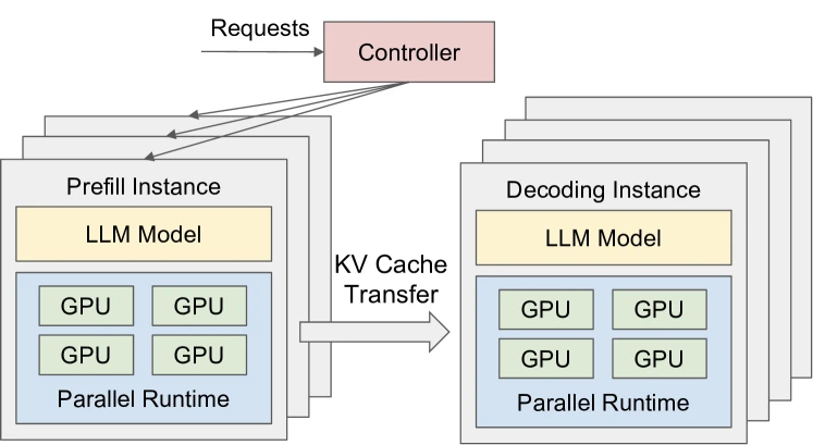
Figure 6 of DistServe (arXiv:2401.09670) — runtime architecture, reproduced for editorial coverage.

5A: DistServe

From the paper, DistServe is structured as three components: a placement algorithm (offline), a runtime (online), and an instance type system (prefill instances and decoding instances).

Instance types. A prefill instance runs the forward pass for prompts only; a decoding instance runs autoregressive generation only. Each instance can use any combination of tensor parallelism (TP) and pipeline parallelism (PP) chosen independently from the other phase.

Runtime architecture (Figure 6). From the paper: requests arrive at a centralised controller, are dispatched to the prefill instance with the shortest queue, the prefill instance computes and stores the KV cache for the prompt, then forwards a metadata handle to the least-loaded decoding instance. The decoding instance pulls the KV cache from the prefill instance’s GPU memory as needed.

KV cache transfer protocol. From the paper, the protocol is pull-based, not push-based: “decoding instances fetch KV cache from prefill instances as needed, using the GPU memory of prefill instances as a queuing buffer.” When the cluster has high node-affinity (prefill and decode instances colocated on the same node), the transfer uses NVLink (~600 GB/s). When affinity is low, the transfer goes over network (25 Gbps in the paper’s setup), which dominates cost unless mitigated.

Placement algorithm. From the paper, two placement algorithms handle the two cluster topologies (Algorithm 1 for high node-affinity, Algorithm 2 for low node-affinity). The algorithm enumerates feasible (TP, PP) combinations for prefill and decode independently, simulates each, then replicates instances to meet a target traffic rate. Complexity for Algorithm 1: $O(NM^2)$ with $N$ = node count and $M$ = GPUs per node.

[Adapted] DistServe inherits PagedAttention ⁸ from vLLM for KV-cache memory layout, but adds the cross-instance pull protocol on top. The disaggregation pattern itself is [New].

Figure 10 of DistServe (arXiv:2401.09670) — KV-cache transmission overhead, reproduced for editorial coverage.

5B: Splitwise

From the paper, Splitwise is structured around three machine pools: a prompt pool, a token pool, and a dynamic mixed pool that absorbs load imbalance.

Scheduler design. From the paper, the system runs a Cluster-Level Scheduler (CLS) and per-machine Machine-Level Schedulers (MLS).

• CLS uses Join-the-Shortest-Queue (JSQ) routing to pair an incoming request with a (prompt machine, token machine) tuple.
• CLS rebalances the prompt and token pools when their queue lengths diverge significantly, moving machines into or out of the mixed pool.
• Prompt MLS schedules FCFS, capped at 2048 total tokens per batch (the paper’s chosen prompt-batch cap for throughput-vs-latency).
• Token MLS schedules FCFS with aggressive batching up to GPU memory limits.
• Mixed-pool MLS prioritises prompt work and preempts ongoing token generation when needed.

KV-cache transfer optimisation. From the paper, the critical optimisation is layer-wise asynchronous transfer that overlaps KV-cache movement with continued prompt computation:

“Splitwise triggers an asynchronous transfer of the KV-cache for that layer while the prompt computation continues to the next layer.”

For prompts smaller than 512 tokens on H100, the paper finds serialised transfer is sufficient. For larger prompts, the per-layer transfer reduces observable overhead to 0.8% of E2E latency versus 64% for naive serialised transfer.

Hardware mixing strategy. From the paper, four configurations are evaluated.

Design	Prompt machine	Token machine	Rationale
Splitwise-HH	H100	H100	Homogeneous baseline
Splitwise-AA	A100	A100	Homogeneous, cost-optimised
Splitwise-HA	H100	A100	Compute for prefill, efficient memory for decode
Splitwise-HHcap	H100	H100 (70% power cap)	Power-efficient token generation

The HA and HHcap configurations exist because token generation is insensitive to power capping above ~50% (from Splitwise Figure 9), so the operator can save power or money on the decode side without losing throughput.

[Adapted] Splitwise borrows the continuous-batching scheduling pattern for within-phase batching but applies it independently to each pool. The mixed-pool dynamic rebalancing is [New] relative to DistServe, which keeps phase assignments static once planned.

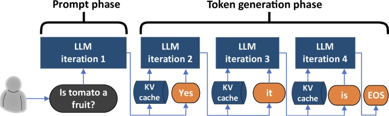
Figure 1 of Splitwise (arXiv:2311.18677) — phase characterisation, reproduced for editorial coverage.

5C: What the two systems share

Both systems split the autoregressive request lifecycle at the prefill/decode boundary, transfer the KV cache to a decode-side GPU, and schedule the two pools independently. Both pull the KV-cache transfer cost down to under 1% of E2E latency via overlap with computation or fast interconnect. Both treat prefill instances and decode instances as having different parallelism degrees in their planners.

The differences are in scope. DistServe optimises a goodput metric under SLO and emphasises the placement algorithm; Splitwise optimises throughput/cost/power jointly and emphasises hardware heterogeneity and dynamic pool rebalancing. [Analysis] In a production deployment, the two contributions are complementary: use DistServe’s placement-search approach with Splitwise’s heterogeneous-pool option and dynamic mixed-pool fallback.

Section 6: Mathematical contributions

The mathematical content of both papers sits in the analytic latency models DistServe uses for its placement simulator. Splitwise relies on empirical measurements rather than analytic models, so the math entries below come primarily from DistServe.

MATH ENTRY 1: Prefill latency model

• Source: DistServe Section 4.2 / Algorithm 1 simulator
• What it is: a closed-form estimate of how long the prefill phase takes for a batch of requests, used by the placement-search simulator to evaluate candidate configurations without running them.
• Formal definition:

$T_{\text{prefill}} = C_1 \cdot (4 t h^2 + 2 t h m) + C_2 \cdot \frac{3 h t_2}{b} + C_3$

• Term-by-term:

  • $t$ is the total number of tokens across the batch (sum of prompt lengths). Units: tokens.
  • $h$ is the hidden dimension of the transformer (e.g., 5120 for OPT-13B). Units: scalar.
  • $m$ is the FFN intermediate dimension (typically $4h$). Units: scalar.
  • $t_2$ is the sum of squared prompt lengths $\sum_i L_i^2$, capturing the quadratic cost of the attention term. Units: tokens².
  • $b$ is the block size (number of tokens grouped together in the attention kernel). Units: tokens.
  • $C_1, C_2, C_3$ are hardware-specific constants fit empirically from microbenchmarks of the target GPU on the target model.
  • The first term $(4 t h^2 + 2 t h m)$ counts the FLOPs of the QKV projection plus FFN; the second term scales the attention cost by the quadratic-in-prompt-length factor; $C_3$ absorbs fixed kernel-launch overhead.

• Worked numerical example: take $h = 4096$, $m = 4h = 16384$, batch of two requests with $L_1 = 256, L_2 = 512$, so $t = 768$ and $t_2 = 256^2 + 512^2 = 65{,}536 + 262{,}144 = 327{,}680$, with $b = 16$ and constants (illustrative) $C_1 = 10^{-13}$ s/FLOP, $C_2 = 10^{-13}$ s/FLOP, $C_3 = 0.001$ s.

  • First term: $4 t h^2 + 2 t h m = 4 \cdot 768 \cdot 4096^2 + 2 \cdot 768 \cdot 4096 \cdot 16384$ FLOPs. The first sub-term is $4 \cdot 768 \cdot 16{,}777{,}216 = 5.15 \cdot 10^{10}$ FLOPs; the second is $2 \cdot 768 \cdot 4096 \cdot 16384 = 1.03 \cdot 10^{11}$ FLOPs. Sum: $\approx 1.55 \cdot 10^{11}$ FLOPs. Multiplied by $C_1 = 10^{-13}$ gives $\approx 0.0155$ s.
  • Second term: $3 h t_2 / b = 3 \cdot 4096 \cdot 327{,}680 / 16 = 2.52 \cdot 10^{8}$ FLOPs. Multiplied by $C_2 = 10^{-13}$ gives $\approx 0.0000252$ s, negligible at these prompt lengths but rises quadratically.
  • Third term: $C_3 = 0.001$ s.
  • Total $T_{\text{prefill}} \approx 0.0166$ s, dominated by the FFN/QKV term.

• Role: the simulator uses this to score candidate (TP, PP) configurations for prefill instances without actually launching them, enabling exhaustive search.

• Edge cases: at very long prompts ($L \gtrsim 4096$), the $t_2$ attention term dominates and the formula’s accuracy depends on how the production kernel handles flash-attention or other linear-in-memory attention variants. The paper validates the model accuracy at <2% SLO-attainment error against ground truth (Table 2).

• Novelty: [Adapted] from standard transformer FLOP counts. The placement-simulator usage is [New].

• Transferability: [Analysis] reusable for any transformer-FLOP-based serving simulator, with constants re-fit per hardware.

• Why it matters: lets the placement algorithm enumerate hundreds of candidate configurations in seconds rather than running each for minutes.

MATH ENTRY 2: Decode latency model

• Source: DistServe Section 4.2
• What it is: a closed-form estimate of how long one decode step takes for a batch of $t$ active sequences.
• Formal definition:

$T_{\text{decode}} = C_4 \cdot (4 h^2 + 2 h m) + C_5 \cdot 3 h t$

• Term-by-term:

  • $h, m$ as above.
  • $t$ is the number of active sequences in the decode batch (one new token per sequence per step). Units: sequences.
  • $C_4, C_5$ are hardware constants fit empirically.
  • First term: per-step weight read cost (independent of batch size, the weights are read once per step regardless of $t$). This is the memory-bound term that motivates large decode batches.
  • Second term: attention-over-cache cost, linear in active batch size.

• Worked numerical example: same $h = 4096, m = 16384$, batch $t = 32$ active decodes, $C_4 = 10^{-13}, C_5 = 10^{-13}$.

  • First term: $4 \cdot 4096^2 + 2 \cdot 4096 \cdot 16384 = 6.71 \cdot 10^{7} + 1.34 \cdot 10^{8} = 2.01 \cdot 10^{8}$ FLOPs. Multiplied by $C_4$: $2.01 \cdot 10^{-5}$ s = 20 μs.
  • Second term: $3 \cdot 4096 \cdot 32 = 3.93 \cdot 10^{5}$ FLOPs. Multiplied by $C_5$: $3.93 \cdot 10^{-8}$ s ≈ 0.04 μs. Negligible.
  • Total per-step decode latency $\approx 20$ μs. Note this is FLOP-derived; in practice decode is memory-bandwidth-bound, so the empirical constants $C_4, C_5$ absorb the bandwidth cost.

• Role: lets the simulator estimate TPOT for any candidate decode-instance configuration.

• Edge cases: at very large $t$, the attention-over-cache term grows linearly while the weight-read term stays constant, past some break-even batch size, decode becomes attention-bound rather than weight-read-bound. Modern flash-attention variants push the break-even higher.

• Novelty: [Adapted] from standard transformer FLOP counts. The decoupling of decode-instance constants from prefill-instance constants is the contribution.

• Transferability: [Analysis] same constants do not generally transfer across (model, hardware) pairs; the simulator must re-fit.

• Why it matters: the fact that the leading $T_{\text{decode}}$ term is independent of batch size is the mathematical reason decode wants large batches and prefill does not.

MATH ENTRY 3: Goodput metric

• Source: DistServe Section 3
• What it is: the optimisation target the whole DistServe paper is built around. Throughput-with-SLO-filter.
• Formal definition (paraphrased from the paper’s prose):

$G = \max \{ R \mid \Pr[\text{TTFT} < \text{SLO}_{\text{TTFT}} \land \text{TPOT} < \text{SLO}_{\text{TPOT}}] \geq \alpha \} / N_{\text{GPU}}$

• Term-by-term:
  • $R$ is the offered request rate (requests/second).
  • The probability is taken over the workload distribution and the scheduler’s stochastic behaviour.
  • $\alpha$ is the SLO attainment target (commonly 0.9 = P90 or 0.99 = P99).
  • $N_{\text{GPU}}$ is the GPU count in the deployment.
• Worked numerical example: a deployment of 8 A100 GPUs sustains $R = 4$ req/s while keeping 92% of requests under the joint SLO at $\alpha = 0.9$. Goodput $G = 4 / 8 = 0.5$ req/s/GPU. If a competing deployment of 8 A100s sustains only $R = 1.6$ req/s under the same SLO, its goodput is $0.2$ req/s/GPU. DistServe claims $2.5\times$ improvement in this case.
• Role: the metric every placement-search configuration is scored against.
• Edge cases: if no candidate configuration meets $\alpha$ at any $R > 0$, the SLO is infeasible at the cluster scale and the operator must add GPUs.
• Novelty: [Adapted] the goodput concept exists in networking literature; DistServe’s contribution is applying it as the placement-search objective for LLM serving.
• Transferability: [Analysis] directly portable to any serving system that exposes a workload distribution and SLO pair.
• Why it matters: throughput-only optimisation rewards configurations that violate SLO; goodput corrects this.

MATH ENTRY 4: KV-cache size per request

• Source: standard transformer accounting (both papers reference this implicitly without restating the formula).
• What it is: how much GPU memory the KV cache occupies for a single request with prompt length $L$ and current generation position $g$.
• Formal definition:

$\text{KV size} = 2 \cdot (L + g) \cdot n_{\text{layers}} \cdot n_{\text{heads}} \cdot d_{\text{head}} \cdot \text{bytes per element}$

• Term-by-term:

  • The leading $2$ is for K and V (one tensor each).
  • $n_{\text{layers}}, n_{\text{heads}}, d_{\text{head}}$ are model-architecture constants. $n_{\text{heads}} \cdot d_{\text{head}} = h$ for standard multi-head attention; for grouped-query attention (GQA) the active head count is smaller.
  • Bytes per element: 2 for FP16/BF16, 1 for FP8 or INT8 cache quantisation.

• Worked numerical example: OPT-13B has $n_{\text{layers}} = 40, n_{\text{heads}} = 40, d_{\text{head}} = 128, h = 5120$. For a request with $L = 1024$ tokens at the moment prefill completes:

  $\text{KV size} = 2 \cdot 1024 \cdot 40 \cdot 40 \cdot 128 \cdot 2 \text{ bytes} = 838{,}860{,}800 \text{ bytes} \approx 800 \text{ MB}$

  This is the volume that must be transferred from prefill GPU to decode GPU when the request migrates.

• Role: determines KV-cache transfer latency and the GPU memory budget per concurrent request.

• Edge cases: the cache grows as decode proceeds; the transfer between prefill and decode instances captures only the post-prefill state, not the per-step growth. The decode instance grows the cache locally as it generates.

• Novelty: standard.

• Transferability: directly portable.

• Why it matters: a 1024-token prompt produces ~800MB of KV cache. Over NVLink at 600 GB/s, that’s ~1.3 ms; over 25 Gbps Ethernet that’s ~256 ms. The two papers’ KV-transfer optimisations are about hiding this latency.

Section 7: Algorithmic contributions

ALGORITHM ENTRY 1: DistServe placement search (Algorithm 1, high node-affinity)

• Source: DistServe Section 4.2
• Purpose: find the (TP, PP) configuration that maximises per-GPU goodput for a given model, workload, and SLO.
• Inputs: model architecture, workload distribution $(L, O)$, SLO pair $(\text{SLO}_{\text{TTFT}}, \text{SLO}_{\text{TPOT}}, \alpha)$, node count $N$, GPUs per node $M$, target traffic rate $R$.
• Outputs: chosen (TP, PP) for prefill instances; chosen (TP, PP) for decode instances; replication counts for each instance type.
• Pseudocode (reproduced from the paper’s prose description; rendered as a PNG body figure further in this section for the headline algorithm):

for intra_op ∈ {1, 2, …, M}:
  for inter_op ∈ {1, 2, …, N×M / intra_op}:
    if model_size / (inter_op × intra_op) < GPU_memory:
      parallelise model with (intra_op = TP, inter_op = PP)
      simulate prefill_goodput  using prefill latency model (MATH ENTRY 1)
      simulate decode_goodput   using decode latency model (MATH ENTRY 2)
      track (TP, PP) that maximises per-GPU goodput for each phase
replicate the best prefill and decode instances to meet target rate R
return placement plan

• Hand-traced example on minimal input: take $N=2, M=4$ (a small cluster of two 4-GPU nodes), model OPT-13B fitting on one GPU.

  • Iteration $\text{intra\_op}=1, \text{inter\_op}=1$: a single-GPU prefill instance. Simulator runs MATH ENTRY 1 with the workload’s distribution of $L$. Suppose it returns prefill goodput 1.0 req/s. Track this as best so far for prefill.
  • Iteration $\text{intra\_op}=1, \text{inter\_op}=2$: a 2-GPU pipeline-parallel prefill instance across one node. Simulator estimates higher prefill throughput per instance but two GPUs used; per-GPU goodput may not improve. Suppose it returns 0.9 req/s/GPU. Worse, keep the previous best.
  • Iteration $\text{intra\_op}=2, \text{inter\_op}=1$: a 2-GPU tensor-parallel prefill instance. Simulator returns 1.4 req/s/GPU. Update best to TP=2, PP=1.
  • Continue enumerating up to the cluster limit.
  • Repeat the same loop for decode goodput, fitting MATH ENTRY 2.
  • Final replication: if target $R = 8$ req/s and best prefill is 1.4 req/s/GPU on a 2-GPU TP instance, the planner replicates the prefill instance ceil(8 / 2.8) = 3 times = 6 GPUs. The remaining 2 GPUs go to decode replication.

• Complexity: $O(NM^2)$ in the enumeration, dominated by the inner simulator calls. From the paper (Figure 12): under 1.3 minutes for the largest evaluated setting, scaling linearly with CPU cores.

• Hyperparameters: workload-profile granularity, SLO confidence target $\alpha$, simulator step size.

• Failure modes: if no configuration meets $\alpha$ at the requested $R$, the algorithm returns infeasible and the operator must add cluster capacity.

• Novelty: [New] as applied to prefill-decode disaggregated planning. The enumeration pattern itself is standard in distributed-systems literature.

• Transferability: [Analysis] reusable for any LLM serving system that exposes (TP, PP) as configurable parameters and has analytic latency models.

ALGORITHM ENTRY 2: Splitwise CLS rebalancing

• Source: Splitwise Section IV (Scheduler design)
• Purpose: keep the prompt pool and token pool size matched to actual workload demand, using the mixed pool as a buffer.
• Inputs: queue lengths $q_{\text{prompt}}, q_{\text{token}}$, machines $\mid \mathcal{M}_{\text{prompt}}\mid , \mid \mathcal{M}_{\text{token}}\mid , \mid \mathcal{M}_{\text{mixed}}\mid$, rebalancing thresholds.
• Outputs: pool reassignments (machine $\to$ pool).
• Pseudocode (reconstructed from the paper’s prose; the paper does not present formal pseudocode for CLS):

on every arrival:
  pair = JSQ(machine in M_prompt, machine in M_token)
  dispatch request to pair

every Δt seconds (rebalancing tick):
  if q_prompt / |M_prompt| > τ_high and q_token / |M_token| < τ_low:
    move one machine from M_token (or M_mixed) into M_prompt
  if q_token / |M_token| > τ_high and q_prompt / |M_prompt| < τ_low:
    move one machine from M_prompt (or M_mixed) into M_token
  if both queues balanced:
    consolidate machines into M_mixed to absorb future imbalance

• Hand-traced example on minimal input: cluster of 4 machines, initial split $\mathcal{M}_{\text{prompt}} = \{A, B\}, \mathcal{M}_{\text{token}} = \{C, D\}, \mathcal{M}_{\text{mixed}} = \emptyset$.

  • Step 1: a burst of long-output coding-style requests arrives. The token queue grows, $q_{\text{token}}$ rises while $q_{\text{prompt}}$ stays low.
  • Step 2: at the rebalance tick, the threshold $\tau_{\text{high}}$ is crossed on token-pool queue ratio. CLS moves machine $B$ from prompt pool to token pool. New state: $\mathcal{M}_{\text{prompt}} = \{A\}, \mathcal{M}_{\text{token}} = \{B, C, D\}$.
  • Step 3: workload mix shifts back to balanced. Queues equalise. At next rebalance tick, CLS moves $B$ into $\mathcal{M}_{\text{mixed}}$ as a buffer rather than back to prompt.
  • Step 4: a new burst of conversation traffic arrives. $\mathcal{M}_{\text{mixed}}$ absorbs the prompt overflow via preemptive prompt-priority scheduling on $B$.

• Complexity: per-tick work is $O(\mid \mathcal{M}\mid )$ to evaluate queue ratios and pick a machine to move.

• Hyperparameters: rebalance tick $\Delta t$, low/high thresholds $\tau_{\text{low}}, \tau_{\text{high}}$. The paper does not report exact tuning values in the abstract content surfaced; this is a [Reconstructed] gap.

• Failure modes: rapid workload-mix swings within shorter than $\Delta t$ cause oscillation; the mixed pool absorbs this in steady state.

• Novelty: [New], the dynamic mixed pool is the distinguishing Splitwise contribution.

• Transferability: [Analysis] portable to any multi-pool inference cluster.

ALGORITHM ENTRY 3: Layer-wise asynchronous KV-cache transfer (Splitwise)

• Source: Splitwise KV-cache transfer optimisation section
• Purpose: overlap KV-cache transfer with continued prefill computation, hiding the transfer cost.
• Inputs: model with $L$ layers, prompt to prefill, source (prompt) machine, destination (token) machine.
• Outputs: completed prefill on source, fully transferred KV cache on destination.
• Pseudocode (reconstructed from the paper’s prose):

for layer ℓ = 1 to L:
  compute attention(layer ℓ) on prompt machine
  produce K_ℓ, V_ℓ
  async send (K_ℓ, V_ℓ) to token machine via InfiniBand
  (transfer happens concurrently with computation of layer ℓ+1)
wait for first output token from layer L on prompt machine
emit first token to client
ensure all async transfers have completed before handing off to token machine

• Hand-traced example on minimal input: model with 4 layers, prompt of 1024 tokens. Suppose each layer’s prefill compute takes 5ms and each layer’s KV transfer takes 3ms.

  • $t=0$: start compute layer 1.
  • $t=5$ms: layer 1 compute done, $K_1, V_1$ produced. Start async transfer of $K_1, V_1$ (will finish at $t=8$ms). Start compute layer 2.
  • $t=8$ms: $K_1, V_1$ delivered to token machine.
  • $t=10$ms: layer 2 compute done. Start async transfer of $K_2, V_2$ (will finish at $t=13$ms). Start compute layer 3.
  • $t=13$ms: $K_2, V_2$ delivered.
  • $t=15$ms: layer 3 compute done. Start async transfer.
  • $t=18$ms: $K_3, V_3$ delivered.
  • $t=20$ms: layer 4 compute done. Start async transfer.
  • $t=23$ms: $K_4, V_4$ delivered. Handoff complete.

  Total wall-clock: 23ms. Naive serialised would have been $4 \cdot 5 + 4 \cdot 3 = 32$ms. The overlap saved 9ms (~28%). For longer prompts and deeper models the savings compound; the paper reports 0.8% E2E versus 64% naive for production-scale prompts.

• Complexity: same FLOP count as colocated; the transfer cost reduces to the last layer’s $K_L, V_L$ transfer that cannot be overlapped.

• Hyperparameters: layer granularity (per-layer vs grouped-layer), threshold below which serialised transfer is used (the paper notes <512 tokens on H100).

• Failure modes: if InfiniBand bandwidth is below the per-layer transfer rate, the transfer cannot keep up with compute and queues at the source.

• Novelty: [New] as applied to LLM-serving disaggregation. The compute-communication overlap pattern itself is decades old in HPC.

• Transferability: [Analysis] applies to any layer-structured network with a layer-by-layer cacheable state.

[Algorithm 1 of DistServe (arXiv:2401.09670), the placement-search procedure, is reproduced visually as a PNG body figure further down this article for at-a-glance reference.]

Section 8: Specialised design contributions

Subsection 8A, LLM / prompt design. Not applicable to this paper. Both DistServe and Splitwise are serving-system papers; the LLM is a fixed-weight artefact being served, not a designed prompt pipeline.

Subsection 8B, Architecture-specific details.

• DistServe relies on PagedAttention for KV-cache memory layout, inherited from vLLM. The disaggregation does not change the per-instance attention implementation.
• Splitwise deliberately runs token generation on memory-bandwidth-optimised hardware (A100 or power-capped H100) while running prefill on compute-dense hardware (full-power H100). The architecture-specific insight: the A100’s 1.55 TB/s HBM bandwidth is closer to the H100’s 3.35 TB/s than the A100’s 312 TFLOPS is to the H100’s 1979 TFLOPS, so for memory-bound decode the A100 is the cost-effective choice.

Subsection 8C, Training specifics. Not applicable to this paper. Neither paper trains a model.

Subsection 8D, Inference / deployment specifics.

• DistServe recommends placing prefill and decode of the same model stage on the same node when intra-node NVLink is available, reducing the KV-transfer cost to ~1 ms for OPT-175B.
• Splitwise recommends an InfiniBand fabric between prompt and token pools at 200-400 Gbps. The paper suggests RoCE as a fallback but flags it as an open question.
• Neither paper addresses speculative decoding or parallel sampling; both target the standard autoregressive serving pattern.

Section 9: Experiments and results

DistServe evaluation

Datasets. From the paper:

• ShareGPT (chatbot): variable input/output, real conversational distribution.
• HumanEval (code completion): short prompts.
• LongBench (summarisation): long documents, long outputs.

Hardware. 4 nodes × 8 NVIDIA A100-80GB GPUs each, NVLink intra-node (600 GB/s), 25 Gbps cross-node.

Models. OPT-13B (26 GB), OPT-66B (132 GB), OPT-175B (350 GB).

Baseline. vLLM with PagedAttention and continuous batching.

SLO targets (from the paper). Chatbot: TTFT 0.2s / TPOT 0.1s for 13B. Code completion: TTFT 0.125s. Summarisation: TTFT 15s / TPOT 0.15s.

Main results at 90% SLO attainment.

Workload	Model	DistServe vs vLLM (90% SLO)
Chatbot	OPT-13B	2.0×-3.41× higher sustainable request rate
Code completion	OPT-66B	3.2× higher request rate, 1.5× tighter SLO
Summarisation	OPT-66B	4.48× higher request rate, 10.2× tighter SLO

Numbers reproduced From the paper, Figures 8-9. ⁹

Ablation (Figure 11). Stripping the placement-search component (DistServe with no parallelism search) closes most of the gap to vLLM. The disaggregation pattern alone delivers most of the gain; the placement search captures the last 1.3-1.5×.

KV-cache transfer cost (Figure 10). For OPT-175B, transmission overhead is <0.1% of total latency when NVLink-colocated, and 95% of requests see <30ms transmission delay even in the cross-node configuration.

Simulator accuracy (Table 2). <2% error between simulated and measured SLO attainment across rates 1.0-4.0 req/s.

Algorithm runtime (Figure 12). Under 1.3 minutes for the largest setting; scales linearly with CPU cores.

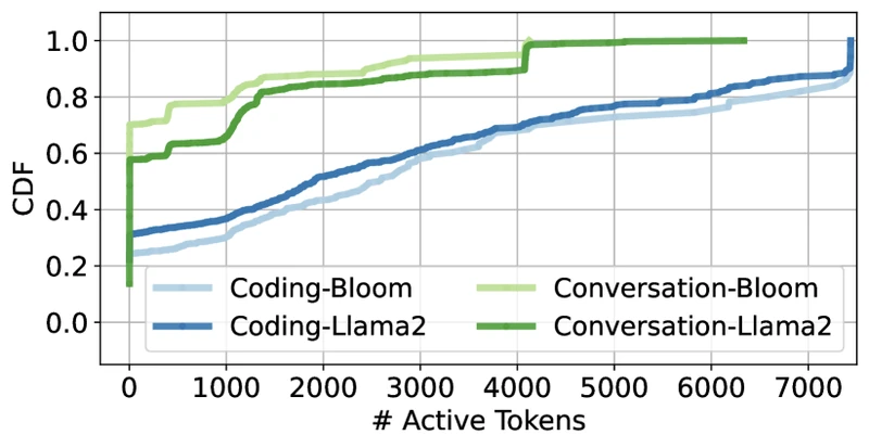
Figure 4 of Splitwise (arXiv:2311.18677) — batched-token distribution, reproduced for editorial coverage.

Splitwise evaluation

Models. BLOOM-176B (70 layers, hidden size 14336) and Llama2-70B (80 layers, hidden size 8192).

Workload traces. Production Azure traces representing two services: a coding service (median 1500 input tokens, 13 output tokens) and a conversation service (median 1020 input tokens, 129 output tokens).

Hardware. 2× DGX-A100 plus 2× DGX-H100 machines connected via InfiniBand (200 Gbps for A100, 400 Gbps for H100).

SLOs. P50/P90/P99 latency targets for TTFT, time-between-tokens (TBT), and E2E (paper’s Table VI).

Main results.

Configuration	Iso-power	Iso-cost	Result
Splitwise-AA	28 kW budget	–	2.15× throughput vs Baseline-A100
Splitwise-HA	28 kW budget	–	1.18× throughput vs Baseline-H100 at 10% lower cost
Splitwise-AA	–	matched cost	1.4× throughput vs Baseline-H100 at 20% lower cost
Splitwise-HHcap	28 kW budget	cost-optimised	Same throughput as Baseline-H100 at 25% lower power

Numbers reproduced From the paper. ¹⁰

Critical insights from characterisation. From the paper:

• Prompt phase utilises compute efficiently; token phase remains memory-bound despite batching.
• 60-70% of E2E wall time is spent in token generation with relatively small batch sizes.
• Prompt throughput degrades after 2048 tokens; token throughput scales linearly with batch size up to memory limits.
• Token phase insensitive to power caps above 50%, the empirical justification for HHcap.

Independent benchmark cross-checks

[External comparison] As of May 2026, independent reproducibility data points include:

• vLLM’s own disaggregated-prefilling documentation ⁵ states explicitly: “Disaggregated prefill DOES NOT improve throughput.” This is consistent with both papers’ framing: the benefit is in tail-latency and goodput at fixed throughput, not raw tokens/second.
• NVIDIA Dynamo ⁶ ships disaggregation as a first-class architectural option, citing both papers in its design notes.
• Mooncake (Moonshot AI’s Kimi) ⁷ reports production deployment of a related disaggregated KV-cache pattern at scale, with separate emphasis on KV-cache pooling.

[Analysis] No independent reproducibility study of DistServe’s 4.48× number has been published as of the cited fetch date; the SOTA claim is the authors’ framing on their chosen benchmark suite. Splitwise’s iso-cost throughput claim is similarly the authors’ framing and depends on assumed A100/H100 price ratios that drift with market conditions.

Evidence audit

• Strongly supported (From the papers). The qualitative claim that disaggregation reduces TTFT/TPOT interference and yields goodput gains under stringent SLOs. Both papers’ ablations and characterisations directly support this.
• Partially supported. The exact magnitude of the gain. Both papers report large multipliers (4.48×, 2.15×) that depend on workload mix, SLO tightness, and hardware ratios. The qualitative direction generalises; the multiplier does not.
• Narrow evidence. Heterogeneous-hardware claims (HA, HHcap) rest on Splitwise’s specific A100/H100 ratio. Newer hardware (B100, MI300X) changes the calculus.

Section 10: Technical novelty summary

Component	Type	Novelty level	Justification	Source
Phase-disaggregated serving architecture	Architecture	Combination novel	Splits a known transformer-inference workload into known phases on known parallelism strategies; the disaggregation pattern as applied to LLM serving is the contribution	DistServe Section 3; Splitwise Section IV
Goodput-as-placement-objective	Method	Incrementally novel	Goodput exists in networking; first-class use as the LLM-serving placement objective is new	DistServe Section 3
Pull-based KV-cache transfer	Method	Fully novel	The pull-with-prefill-as-queuing-buffer protocol is DistServe-specific	DistServe Section 4
Layer-wise async KV transfer	Method	Fully novel	The compute-communication overlap pattern adapted to per-layer KV transfer in LLM serving	Splitwise §IV
Dynamic mixed pool	Method	Fully novel	The triple-pool (prompt / token / mixed) load-rebalancing scheme	Splitwise §IV
Heterogeneous hardware mixing (HA, HHcap)	Deployment	Combination novel	Different GPU types per phase; H100/A100 split	Splitwise §VI
Placement-search algorithm (enumerate + simulate + replicate)	Algorithm	Incrementally novel	Enumeration is standard; the latency-model-driven simulator and goodput target are novel composition	DistServe Algorithm 1
Prefill/decode analytic latency models	Math	Adopted	Standard transformer FLOP counts re-applied as planner inputs	DistServe Section 4
PagedAttention	Architecture	Adopted	Inherited from Kwon et al. 8	vLLM, SOSP 2023
Continuous batching	Scheduling	Adopted	Standard for in-pool batching, applied per-phase	Multiple prior systems

Single most novel contribution. [Analysis] The disaggregation pattern itself, treating prefill and decode as workloads that should run on different machines, is the conceptual contribution that has propagated. Specific mechanisms (pull-based transfer, layer-wise overlap, mixed pool) are valuable but smaller. The architectural shift is what every follow-up paper and production framework now treats as the baseline.

What the papers do NOT claim to be novel. PagedAttention, continuous batching within a pool, tensor and pipeline parallelism, FLOP-count latency models, FCFS scheduling, JSQ routing, transformer attention itself.

Section 11: Situating the work

Prior work. Pre-2024 LLM-serving systems, Orca (OSDI 2022), vLLM (SOSP 2023), TensorRT-LLM, Triton Inference Server, share a continuous-batching architecture that mixes prefill and decode steps within a single pool. They optimise throughput under a fixed SLO; none separates the phases.

What these papers change conceptually. Both reframe the problem from “maximise throughput on a homogeneous pool” to “find the configuration that maximises goodput-per-cost across heterogeneous, phase-specialised pools.” [Analysis] This is the right framing because the two phases really are unrelated workloads sharing only the model weights; coupling them was an artefact of the deployment template, not a fundamental requirement.

Contemporaneous related work. [External comparison]

• Sarathi-Serve (Agrawal et al., OSDI 2024) ¹² attacks the same interference problem with chunked prefill rather than phase separation. The two approaches are not mutually exclusive, Sarathi-Serve within a single pool plus DistServe across pools is a defensible production stack.
• SARATHI (Agrawal et al., 2023) ¹¹ is the precursor, introducing chunked prefill + decode piggybacking. Both Sarathi papers and DistServe come from the same OSDI 2024 cycle; the community converged on “stop letting prefill and decode collide” via two different mechanisms.
• Mooncake (Moonshot AI, 2024) ⁷ extends disaggregation to a separate KV-cache pool with cross-request reuse, taking the architectural idea further. Mooncake explicitly cites both DistServe and Splitwise as antecedents.
• NVIDIA Dynamo (2024-2025) ⁶ productises the pattern as a serving-framework abstraction.

[Reviewer Perspective] Strongest skeptical objection. Disaggregation roughly doubles the minimum cluster size and adds an interconnect requirement (NVLink intra-node or InfiniBand inter-node). For low-traffic deployments, a single user, a research demo, a batch-inference pipeline without latency SLOs, colocated serving is strictly simpler and probably faster end-to-end. The two papers’ benefits only materialise at production scale with binding TTFT/TPOT constraints.

[Reviewer Perspective] Author-side rebuttal. Both papers explicitly target production serving with SLOs; neither claims disaggregation is the right pattern at all scales. DistServe’s placement algorithm can in principle return a no-disaggregation configuration if the SLO is loose enough. Splitwise’s mixed pool can absorb the entire workload when the operator only has a few machines.

What remains unsolved.

• Speculative decoding interaction. Both papers assume one decode step per output token. Speculative decoding draws multiple candidate tokens per step and changes the phase boundaries.
• Multi-turn conversation context reuse. Each new turn re-prefills the conversation history; cross-turn KV-cache reuse would change the disaggregation math. [External comparison] Mooncake addresses this directly.
• Heterogeneous hardware automation. Splitwise picks (H100, A100) by hand. A planner that automatically picks the right (compute-class, memory-class) pair per workload is open.

Three future research directions.

1. Intra-GPU disaggregation. Run prefill and decode on different SM partitions of the same GPU rather than on separate GPUs. This would lower the cluster-size doubling overhead. [Reviewer Perspective] Promising but constrained by current GPU scheduling primitives.
2. Partial-prefill disaggregation for multi-turn. In a chat, only the new turn needs prefill; the prior KV cache can stay on the decode side. Cross-turn KV-cache caching combined with disaggregated new-turn prefill is the natural follow-up. [External comparison] Mooncake’s KV-cache pool is one realisation.
3. Disaggregation-aware speculative decoding. The draft model and target model in speculative decoding have natural decode-side affinity; the relationship to prefill disaggregation has not been studied in depth.

Section 12: Critical analysis

Strengths

• DistServe presents a clean separation of concerns: the placement algorithm is offline and uses analytic models; the runtime is straightforward FCFS routing. The simulator’s <2% error against ground truth (Table 2) makes the offline planning defensible.
• Splitwise delivers the strongest practical contribution: the layer-wise asynchronous KV transfer reduces transfer overhead from 64% to 0.8% of E2E. The hardware-mixing analysis is the most actionable for capacity planners.
• Both papers report large gains under realistic SLOs on real workload distributions. The qualitative direction (disaggregation helps under stringent SLOs) is robust across both papers’ independent setups.

Weaknesses explicitly stated by the authors

• DistServe (Section 8 / conclusion). Fault tolerance is not implemented; a fault in one decoding instance mapped to multiple prefill instances could propagate. Preemption is feasible in the architecture but not implemented. Non-autoregressive generation is out of scope.
• Splitwise (limitations). Interconnect assumes InfiniBand availability; RoCE suggested as fallback but not evaluated. Heterogeneous designs (HA, HHcap) show 7% throughput loss when switching workload types. Hardware scope limited to A100/H100; AMD MI-250 and Intel Sapphire Rapids untested. Server-side conversation-context caching is not modelled.

Weaknesses not stated or understated by the authors

[Reviewer Perspective]

• Neither paper deeply addresses the cluster-size doubling. A 1-GPU deployment cannot disaggregate; the minimum useful cluster is at least 2 GPUs (one prefill, one decode) and realistically more for SLO compliance. For small operators or single-tenant deployments, this is a non-trivial cost.
• Both papers benchmark against vLLM as the colocated baseline. Sarathi-Serve ¹² was a contemporaneous competitor offering a different solution to the same problem. The papers do not directly compare against Sarathi-Serve, which leaves the question “which is better, chunked prefill or phase disaggregation?” open. [External comparison] Production frameworks like Dynamo ⁶ support both patterns, suggesting the right answer is workload-dependent.
• DistServe’s placement algorithm assumes a stationary workload distribution. Real production traffic has bursts, time-of-day effects, and incident-driven traffic shifts. The 4.48× number is a steady-state result; behaviour under traffic shocks is underexplored.
• Splitwise’s heterogeneous designs lose 7% throughput under workload-type changes, flagged in passing in the paper but not investigated as a deployment risk. [Analysis] For operators serving mixed workloads, this is a meaningful caveat.

Reproducibility check

• Code. DistServe code is open-sourced (github.com/LLMServe/DistServe); Splitwise’s evaluation infrastructure is partly described but the production scheduler implementation is not released as of the cited fetch date.
• Data. DistServe uses publicly available ShareGPT, HumanEval, LongBench. Splitwise’s Azure production traces are described in distribution but the raw traces are not released.
• Hyperparameters. DistServe fully specifies SLO targets, simulator constants, and parallelism enumeration ranges. Splitwise specifies SLO targets and prompt-batch caps; some MLS thresholds are not in the abstract content.
• Compute. DistServe reports 4 nodes × 8 A100-80GB. Splitwise reports 2 DGX-A100 + 2 DGX-H100. Both reported.
• Trained model weights. Both papers use publicly released models (OPT, BLOOM, Llama2). No new weights released.
• Evaluation set. Released for DistServe (public benchmarks). Partly released for Splitwise (trace distributions but not raw traces).
• Overall. DistServe: fully reproducible. Splitwise: partially reproducible, the heterogeneous-hardware results require the same A100+H100 cluster setup.

Methodology

Methodology

• Sample size: DistServe, workload distributions sampled from ShareGPT (varies), HumanEval (164 prompts), LongBench (multi-document, varies). Splitwise, two Azure production traces with stated medians but full distribution sizes not reported in the abstract surfaced.
• Evaluation set: DistServe, public benchmarks held-out from training. Splitwise, production Azure traces, distribution-described.
• Baselines: DistServe, vLLM (default), vLLM++ (with parallelism search), DistServe-Low, DistServe-High. Splitwise, Baseline-A100 colocated, Baseline-H100 colocated.
• Hardware/compute: DistServe, 4 nodes × 8 × A100-80GB, NVLink intra, 25 Gbps inter. Splitwise, 2 DGX-A100 + 2 DGX-H100, InfiniBand 200/400 Gbps.

Generalisability

To other models: OPT and BLOOM are dense decoder-only transformers. Mixture-of-experts models change the FLOP-per-token math and the KV-cache size formula; neither paper evaluates MoE. Encoder-decoder models (Flan-T5) have a different phase structure.

To larger scales: DistServe evaluates up to 175B; Splitwise to 176B. Trillion-parameter MoE models (Mixtral 8×22B, DeepSeek-V3) exist outside the evaluation envelope. [Analysis] The qualitative direction should hold but the constants change substantially.

To different backbones: the analytic latency models in DistServe use standard transformer FLOPs; non-standard backbones (Mamba, RWKV) have different decode-step cost structures.

Assumption audit

The known-workload-distribution assumption is the most fragile. Production workloads drift; both papers’ planners are designed for re-running offline, but the cadence and the cost of replanning under drift is underexplored. The InfiniBand/NVLink interconnect assumption is the second-most fragile; cloud-deployed disaggregation over commodity networking is materially harder.

What would make the papers stronger

[Analysis]

• Direct head-to-head comparison against Sarathi-Serve and Mooncake.
• Workload-shift robustness experiments showing degradation under sudden distribution change.
• MoE-model evaluation.
• Cost analysis at current (2026) GPU prices rather than 2023-2024 pricing assumptions.

Section 13: What is reusable for a new study

REUSABLE COMPONENT 1: The disaggregation architectural pattern itself

• What it is: separating prefill and decode onto independent GPU pools with KV-cache transfer between them.
• Why worth reusing: the dominant production pattern as of 2026; supported by vLLM, Dynamo, Mooncake, others.
• Preconditions: at least a 2-GPU cluster with NVLink or InfiniBand between the prefill and decode machines; workload with binding TTFT/TPOT SLOs.
• What would need to change in a different setting: for MoE models, the per-expert routing complicates phase boundaries. For multi-modal models, the prefill phase may include vision-encoder work that has its own scheduling needs.
• Risks: cluster-size doubling overhead at low traffic; transfer-cost amplification on commodity networking.
• Interaction effects: combines naturally with PagedAttention, continuous batching within each pool, and chunked-prefill (Sarathi-Serve) inside the prefill pool.

REUSABLE COMPONENT 2: Goodput-as-placement-objective

• What it is: optimising for max request rate subject to a joint SLO, divided by GPU count.
• Why worth reusing: throughput-only optimisation rewards SLO-violating configurations; goodput corrects this.
• Preconditions: well-defined SLO and workload distribution.
• What would need to change in a different setting: multi-tenant clusters with per-tenant SLOs need a multi-objective extension.
• Risks: defining “SLO attainment” varies (P50? P90? P99?); the metric is sensitive to this choice.
• Interaction effects: pairs naturally with placement search and capacity planning.

REUSABLE COMPONENT 3: Layer-wise asynchronous KV-cache transfer

• What it is: overlapping per-layer KV-cache transfer with continued prompt computation.
• Why worth reusing: reduces transfer cost from dominant to negligible for production-scale prompts.
• Preconditions: layer-structured network with cacheable per-layer state; sufficient interconnect bandwidth.
• What would need to change in a different setting: non-layer-uniform models (mixture-of-depths, recurrent attention) need a different overlap scheme.
• Risks: bandwidth-bound transfers stall the next layer’s transfer; need to monitor for backpressure.
• Interaction effects: pairs with continuous batching within the prefill pool.

REUSABLE COMPONENT 4: Dynamic mixed-pool rebalancing

• What it is: a third pool absorbing workload-mix imbalance via preemptive prompt-priority scheduling.
• Why worth reusing: gives operational headroom for workload drift without re-planning.
• Preconditions: machines capable of running both prefill and decode (no architectural restriction).
• What would need to change in a different setting: for heterogeneous-hardware deployments (HA), only the H100 machines can serve as mixed-pool members effectively.
• Risks: oscillation under rapid workload-mix swings.
• Interaction effects: complements DistServe’s offline placement.

Dependency map. The disaggregation pattern (1) is the architecture; goodput (2) is the metric used to plan it; layer-wise KV transfer (3) hides the transfer cost; mixed-pool rebalancing (4) absorbs workload drift in production. All four are independently useful but reinforce each other in a complete deployment.

Recommendation. [Analysis] For a new study aiming to extend LLM serving:

• Adopt the disaggregation pattern (1) as the baseline.
• Apply the goodput metric (2) as the optimisation target.
• Implement layer-wise async KV transfer (3) if the cluster has InfiniBand or NVLink between pools.
• Defer mixed-pool rebalancing (4) until production traces show workload drift is a real problem.

Type of new study that benefits most. Production-serving systems with stringent SLOs and known workload distributions. Research demos with one model and one tenant get less benefit and the architectural complexity is harder to justify.

Section 14: Known limitations and open problems

Limitations explicitly stated by the authors.

• DistServe. Fault tolerance (single-instance fault can propagate); preemption (architectural support but no implementation); non-autoregressive generation (out of scope).
• Splitwise. InfiniBand assumption (RoCE fallback not evaluated); 7% throughput loss on heterogeneous designs under workload-type shifts; hardware scope limited to NVIDIA A100/H100; conversation-context caching not modelled.

Limitations not stated. [Reviewer Perspective]

• Cluster-size doubling overhead.
• Lack of head-to-head comparison against Sarathi-Serve (DistServe) or Mooncake (both).
• Workload-distribution-drift behaviour under realistic production traffic patterns.
• MoE-model evaluation gap.

Technical root cause of each.

• Cluster-size doubling: a single GPU cannot simultaneously be a prefill instance and a decode instance under either paper’s architecture. Splitwise’s mixed pool partially mitigates this but only for machines large enough to host both roles.
• Sarathi-Serve gap: the two competing OSDI 2024 papers attack the same problem with different mechanisms; the authors of either system had no incentive to benchmark against the other before publication.
• Workload drift: both planners assume stationary distributions.
• MoE gap: both papers were drafted before the MoE-serving wave (Mixtral, DeepSeek-V3); the FLOP/memory accounting differs from dense decoder-only models.

Open problems left behind.

• Optimal phase split for speculative decoding workflows.
• Cross-turn KV-cache reuse interacting with disaggregation (Mooncake’s direction).
• Intra-GPU disaggregation via SM partitioning.
• Cost-aware planner that picks (compute-class, memory-class) hardware pair automatically.
• Disaggregation under cloud-provider commodity networking (RoCE, TCP).

What a follow-up paper would need to solve to address the most critical limitation. The cluster-size doubling overhead is the operational barrier that prevents disaggregation from being a universal recommendation. A follow-up that delivers comparable goodput gains at the same minimum cluster size, e.g., via intra-GPU disaggregation or via dynamic colocation that flips between modes based on load, would generalise the architectural pattern from “production-scale only” to “all-scales recommended.”

How this article reads at three depths

For the curious high-school reader. When you ask a language model a question, the model first reads your whole prompt at once (the “prefill”) and then writes its answer one word at a time (the “decode”). These two steps look very different, one is a big maths problem, the other is many small ones, so two recent research papers, DistServe and Splitwise, argue you should run them on different computers. The result is faster, cheaper LLM serving, especially for chatbot-style apps with strict response-time targets.

For the working developer or ML engineer. Prefill-decode disaggregation is the architectural shift behind vLLM’s experimental disaggregated-prefilling feature, NVIDIA Dynamo, and Mooncake. The headline result: split prefill and decode onto separate GPU pools, transfer the KV cache between them over NVLink or InfiniBand, and you get 2-4× higher sustainable request rate at the same SLO versus colocated vLLM. The trade-offs: minimum cluster size roughly doubles, and you need a fast interconnect to keep KV-transfer cost under 1% of E2E latency. Worth adopting if your workload has binding TTFT/TPOT SLOs at moderate-to-high request rates; overkill for low-traffic deployments. Pair with PagedAttention (still useful within each pool) and consider chunked-prefill (Sarathi-Serve style) inside the prefill pool. vLLM’s docs explicitly note disaggregation does not improve raw throughput; the gain is in tail latency under SLO.

For the ML researcher. DistServe formalises the problem around per-GPU goodput (throughput-with-SLO-filter) and introduces an offline placement-search algorithm that enumerates (TP, PP) configurations for prefill and decode independently, scored by a transformer-FLOP latency simulator with <2% error. The contribution is the goodput-as-objective framing plus the pull-based KV-cache transfer protocol. Splitwise frames the same problem around throughput/cost/power and contributes layer-wise asynchronous KV transfer (reducing overhead from 64% to 0.8% E2E) plus heterogeneous-hardware mixing (H100 prefill + A100 decode). Both share the disaggregation architectural pattern as the load-bearing contribution. Strongest objection: neither paper benchmarks against Sarathi-Serve (chunked prefill, OSDI 2024 contemporaneous), leaving the chunked-prefill-vs-disaggregation question open. Strongest follow-up direction: intra-GPU disaggregation via SM partitioning, which would eliminate the cluster-size doubling overhead that limits the pattern to production-scale deployments.