Vision Encoders: CLIP, SigLIP, EVA-CLIP — Contrastive vs Sigmoid vs Scaling

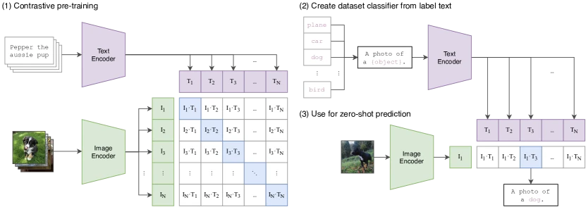
Figure 1 of CLIP (arXiv:2103.00020), reproduced for editorial coverage.

1. Umbrella scope and paper identities

This review covers three artefacts that together codify the dominant recipe for contrastive vision-language pretraining and its successor losses:

• Radford et al. (2021). Learning Transferable Visual Models From Natural Language Supervision (CLIP), arXiv:2103.00020 ¹ . ICML 2021. The paper that established the contrastive image-text recipe at 400M-pair scale and introduced zero-shot classification via prompt embeddings.
• Zhai, Mustafa, Kolesnikov, Beyer (2023). Sigmoid Loss for Language Image Pre-Training (SigLIP), arXiv:2303.15343 ³ . ICCV 2023 Oral. The paper that replaced CLIP’s softmax-normalised InfoNCE loss with an independent pairwise sigmoid loss, removing the global-batch normalisation requirement.
• Tschannen et al. (2025). SigLIP 2: Multilingual Vision-Language Encoders with Improved Semantic Understanding, Localization, and Dense Features, arXiv:2502.14786 ⁵ . The successor recipe that adds captioning, self-distillation, masked prediction, and online data curation on top of the sigmoid loss.
• Sun, Wang, Yu, Cui, Zhang, Zhang, Wang (2024). EVA-CLIP-18B: Scaling CLIP to 18 Billion Parameters, arXiv:2402.04252 ⁶ . The paper that scaled the EVA-CLIP recipe to 18B vision-encoder parameters using only the publicly available LAION-2B and COYO-700M data sources.

Retrieval status: all three primary papers were retrieved from arXiv at draft time and cross-checked against the ICCV 2023 open-access PDF ⁴ for SigLIP. The EVA-CLIP-18B paper does not yet have a venue acceptance noted on arXiv as of 2026-05-19. SigLIP 2 is supplementary context for the SigLIP section; the section’s MATH ENTRY traces SigLIP 1’s loss.

Classification. All four papers fall under: Representation learning · Multimodal · Architecture proposal (each adapts ViT-class encoders) · Training method (loss-function or recipe innovation) · Data-driven. SigLIP 2 and EVA-CLIP-18B additionally classify as Application (multilingual encoders, downstream-VLM backbones).

Primary research questions. CLIP: can natural-language supervision yield a visual representation that transfers to arbitrary downstream tasks without per-task labels? SigLIP: can the global-normalisation requirement of contrastive loss be removed without sacrificing transfer accuracy, and what does that imply for batch-size scaling? EVA-CLIP-18B: how far does the CLIP recipe scale in encoder parameters when initialised from a strong masked-image-modelling (MIM) checkpoint, and is the recipe still data-efficient at 18B parameters?

Core technical claims. CLIP: a single contrastive objective on 400M web image-text pairs produces an encoder competitive with the original supervised ResNet-50 on ImageNet zero-shot ² . SigLIP: a pairwise sigmoid loss achieves higher accuracy than softmax InfoNCE at small batch sizes and matches it at large batch sizes, while removing the all-gather communication that softmax requires ³ . EVA-CLIP-18B: 80.7% average zero-shot top-1 across 27 image-classification benchmarks using only 6B training samples, demonstrating that the EVA initialisation plus LAMB plus FLIP-style masking scales to 18B parameters on open data ⁶ .

Reader prerequisites. High-school algebra is enough to follow the on-ramp. Familiarity with neural-network basics, the dot product, the softmax function, and what a probability distribution is helps but is not required because the Glossary in Section 2.5 covers each of those. Working ML researchers can skip directly to Sections 6 (MATH ENTRY) and 7 (ALGORITHM ENTRY).

2. TL;DR and executive overview

TL;DR (three sentences). CLIP showed that training a vision model to match images with the words that describe them, using 400 million pairs from the web, produces a visual representation that works on tasks the model was never specifically trained for. SigLIP replaced the math used to compare images and text with a simpler version that does not require every batch of training examples to “see” all the others at once, which lets the loss work at very small AND very large batch sizes. EVA-CLIP-18B scaled the original recipe to 18 billion parameters on only publicly-available data and showed that the technique still pays off; accuracy keeps climbing as the model gets bigger.

Executive summary. Vision-language encoders learn to map images and text into a shared geometric space where the embedding of a photograph of a dog sits near the embedding of the words “a photograph of a dog.” CLIP introduced the recipe in 2021 using a contrastive loss that asks the model to score the matching image-text pair higher than every non-matching pair in the same batch. SigLIP swapped that softmax-based scoring for a sigmoid that treats each pair independently, which simplifies the math and the engineering. EVA-CLIP-18B took the original CLIP recipe, added masked-image pretraining as initialisation, and scaled it to 18 billion parameters using LAMB optimisation and FLIP-style image masking. The three papers together describe the dominant design pattern behind modern image-understanding systems ¹⁵ .

Five practitioner-relevant takeaways.

• The contrastive image-text recipe is now the default starting point for visual representation learning on web-scale data. The encoder you ship in production is almost certainly descended from one of these three lines.
• Batch size and global-batch communication dominate the engineering cost of CLIP-style training. SigLIP’s sigmoid loss is the cleanest known fix and is now the default for new public pretraining runs at Google ⁵ .
• Initialisation matters more than the loss function at the largest scales. EVA-CLIP-18B’s 80.7% average is driven heavily by EVA’s masked-image-modelling pretraining, not by changes to the contrastive objective ⁶ .
• Open-data recipes (LAION-2B + COYO-700M) now match or exceed the original CLIP’s closed-data accuracy on standard benchmarks. The argument for proprietary image-text data has weakened, though not vanished.
• The “temperature parameter” in CLIP and the “temperature plus bias” in SigLIP are not minor implementation details. Their initialisation and clipping are load-bearing; mis-tuning them degrades zero-shot accuracy by several points.

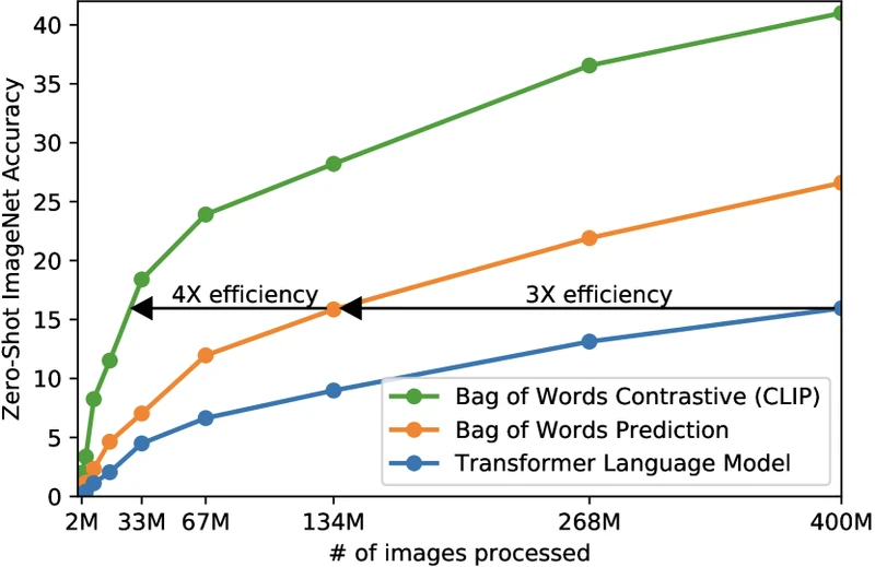
Figure 2 of CLIP (arXiv:2103.00020), reproduced for editorial coverage.

Pipeline overview. At training time, an image encoder (typically a ViT) and a text encoder (typically a Transformer) ingest batches of (image, caption) pairs. The two encoders project into a shared embedding space of fixed dimension $d$ (commonly 512, 768, or 1024). The training objective pulls the embeddings of matching pairs together and pushes non-matching pairs apart. At inference time, classification reduces to embedding each candidate class label as a short prompt (“a photo of a {class}”), embedding the query image, and selecting the class whose text embedding has the highest cosine similarity to the image embedding.

2.5 Glossary

Term	Plain-English explanation	First appears in
Embedding	A list of numbers (a vector) that represents an image or piece of text inside the model. Similar inputs produce similar lists.	Section 2
Cosine similarity	A number between -1 and 1 that measures how aligned two embeddings are; 1 means they point the same direction.	Section 2
Contrastive loss	A training objective that asks the model to score matching pairs higher than non-matching pairs.	Section 2
Softmax	A mathematical operation that turns a list of numbers into a probability distribution (numbers that are positive and sum to 1).	Section 6
Sigmoid	A function that squashes any real number into the range (0, 1); used to compute independent probabilities.	Section 6
InfoNCE	The specific contrastive loss CLIP uses; “Info” because it lower-bounds mutual information, “NCE” because it descends from Noise-Contrastive Estimation.	Section 6
Temperature	A single number $t$ (or $\tau$) the model learns that scales the similarity scores before the loss; controls how “sharp” the distribution is.	Section 6
Batch size	The number of (image, text) pairs the model processes together in one training step.	Section 5
ViT (Vision Transformer)	An image-encoder architecture that splits an image into patches and processes them with a Transformer.	Section 5
Zero-shot classification	Classifying an image into a category the model never saw a labelled training example of, by comparing the image embedding to embeddings of the candidate class names.	Section 2
MIM (masked image modelling)	A self-supervised pretraining task where the model learns to reconstruct hidden patches of an image; EVA’s initialisation strategy.	Section 5
FLIP masking	A trick where the training run drops a fixed fraction of image patches per step, saving compute.	Section 5
LAMB optimizer	A large-batch variant of Adam that normalises updates per layer, used to train EVA-CLIP-18B.	Section 5
[Analysis] label	The publication’s own reasoned assessment, distinct from what the paper itself claims.	Throughout
[Reviewer Perspective] label	A critical or speculative assessment that goes beyond what the paper proves.	Section 11 + 12
[Reconstructed] label	Content the publication faithfully reconstructed because the paper only partially disclosed it.	Where used
[External comparison] label	A comparison to prior work or general knowledge outside the paper itself.	Section 4 + 11
”From the paper:” prefix	Content directly supported by the paper’s text, equations, tables, or figures.	Throughout

3. Problem formalisation

Notation table.

Symbol	Type	Meaning	First appears in
$N$	integer	Number of (image, text) pairs in a training batch	Section 6
$\mathbf{x}_i$	vector in $\mathbb{R}^d$	Image embedding of the $i$-th pair, $L_2$-normalised	Section 6
$\mathbf{y}_j$	vector in $\mathbb{R}^d$	Text embedding of the $j$-th pair, $L_2$-normalised	Section 6
$d$	integer	Shared embedding dimension (CLIP: 512 to 768)	Section 6
$t$ or $\tau$	scalar	Learnable temperature (CLIP stores $\log \tau$; SigLIP stores $\log t$)	Section 6
$b$	scalar	Learnable bias term in SigLIP loss	Section 6
$f_\theta$	function	Image encoder with parameters $\theta$	Section 5
$g_\phi$	function	Text encoder with parameters $\phi$	Section 5
$s_{ij}$	scalar	Similarity $\mathbf{x}_i \cdot \mathbf{y}_j$ between image $i$ and text $j$	Section 6
$z_{ij}$	scalar	SigLIP label: $+1$ when $i = j$, $-1$ otherwise	Section 6
$\mathcal{L}$	scalar	Training loss	Section 6

Formal problem. Given a dataset $\mathcal{D} = \{(I_k, T_k)\}_{k=1}^M$ of $M$ image-text pairs, learn an image encoder $f_\theta: \mathcal{I} \to \mathbb{R}^d$ and a text encoder $g_\phi: \mathcal{T} \to \mathbb{R}^d$ such that for any held-out image $I$ and any set of candidate texts $\{T^{(c)}\}_{c=1}^C$, the index $c^* = \arg\max_c f_\theta(I) \cdot g_\phi(T^{(c)})$ matches the human-judged best caption. The training objective is a function of similarity scores $s_{ij} = f_\theta(I_i) \cdot g_\phi(T_j) / (\lVert f_\theta(I_i) \rVert \lVert g_\phi(T_j) \rVert)$ computed across each training mini-batch of size $N$.

Explicit assumptions. The papers share four assumptions. First, web-crawled image-text pairs are dense enough that a random batch of $N$ pairs contains mostly non-matching combinations. Second, the cosine geometry of the shared embedding space is the right inductive bias; both papers $L_2$-normalise both modalities. Third, a single shared embedding dimension $d$ suffices for both modalities (no asymmetric projection). Fourth, the matching signal at training time generalises to arbitrary text prompts at inference time. [Analysis] Potentially strong assumption: the fourth assumption is the load-bearing one for zero-shot transfer; it relies on the training distribution covering the linguistic forms used in downstream prompts.

Why the problem is hard. The objective requires computing a similarity matrix of size $N \times N$ per batch. For CLIP, $N = 32{,}768$, so each batch step computes $\sim 10^9$ similarities and runs a softmax over a vector of length $N$ for each row and column. The softmax requires an all-reduce across all GPU workers because each worker holds only a slice of the batch; this is the engineering cost SigLIP attacks.

Causal scope. None of the three papers makes a causal claim about the relationship between training data and downstream accuracy. The papers report associational scaling laws: more parameters, more data, and more compute correlate with higher zero-shot accuracy. Whether one of those factors causally drives the others is unaddressed.

Data role. CLIP uses an undisclosed proprietary dataset called WIT (WebImageText) of 400M pairs ² . SigLIP uses Google’s internal WebLI ⁴ . EVA-CLIP-18B uses Merged-2B, the union of LAION-2B and COYO-700M, both publicly available ^{6 12 13} . The data-source asymmetry is one of the few load-bearing differences between the lines.

4. Motivation and gap

Before CLIP, the dominant recipe for visual representation learning was supervised pretraining on ImageNet-1K or ImageNet-21K, followed by per-task fine-tuning. The recipe had three failure modes the paper foregrounds. First, the supervised label set was a closed vocabulary; to add a new class, the practitioner had to gather labelled examples. Second, the recipe required per-task fine-tuning, which is expensive and brittle. Third, supervised pretraining inherits ImageNet’s biases (centre-cropped, single-subject photographs of a curated taxonomy), which limits robustness on domain-shifted test sets.

CLIP’s gap claim is that natural-language captions provide an open vocabulary that scales with the web, removes the per-task fine-tuning step, and includes the linguistic variability the supervised recipe lacks ¹ .

SigLIP’s gap claim is narrower and engineering-focused. Softmax-based InfoNCE requires a global view of the $N \times N$ similarity matrix because the softmax denominator is a sum over the row (or column). On distributed training, this means an all-gather across all workers holding pieces of the batch. The all-gather scales with batch size and dominates communication cost at large $N$. SigLIP’s authors argue that the sigmoid loss removes the requirement because each pair is scored independently ³ .

EVA-CLIP-18B’s gap claim is about scale. Prior open-source CLIP variants (OpenCLIP-G/14 at 1.0B vision parameters ⁸ , EVA-02-CLIP-E/14+ at 4.4B, EVA-CLIP-8B at 7.5B) left open the question of whether the recipe keeps paying off at 10x scale. The paper answers in the affirmative: 18B vision parameters trained on Merged-2B with 6B samples-seen reach 80.7% average across 27 zero-shot benchmarks ⁶ .

[External comparison] Position in the broader landscape: these three lines sit alongside masked-image-modelling backbones (MAE, EVA, DINOv2), captioning-pretrained encoders (CoCa, BLIP-2), and recent unified-encoder models. The CLIP-line’s advantage is the alignment to natural-language prompts at inference, which makes the encoders directly usable as vision-language-model (VLM) front-ends. DINOv2 produces stronger localised features but lacks the text alignment.

5. Method overview

CLIP: original recipe

Architecture. CLIP trained two model families: a ResNet family (ResNet-50, ResNet-101, RN50x4, RN50x16, RN50x64) and a ViT family (ViT-B/32, ViT-B/16, ViT-L/14) ² . The text encoder is a 63M-parameter Transformer with byte-pair-encoded tokens at a 76-token context length. Both encoders project into a 512-dimensional space (768 for the largest ViT) and $L_2$-normalise their outputs.

Training procedure. Adam with decoupled weight decay, batch size 32,768, mixed precision, learnable temperature $\tau$ initialised to $\log(1/0.07)$ and clipped to prevent the logit scale exceeding 100 ² . The largest ViT-L/14 took 12 days on 256 V100 GPUs; the largest ResNet (RN50x64) took 18 days on 592 V100 GPUs. The compute budget is the load-bearing engineering choice that constrains everyone who tried to reproduce CLIP independently.

Inference procedure. Zero-shot classification embeds candidate class names as prompts (the paper found “a photo of a {class}” worked well as a default prompt template) and scores by cosine similarity. Prompt ensembling (averaging embeddings of several prompts per class) adds 1-2 points on most benchmarks.

[Adopted] from prior work: the contrastive image-text idea is not new with CLIP. ConVIRT (Zhang et al. 2020) and earlier multi-modal contrastive work proposed the same shape. CLIP’s contribution is the 400M-pair scale and the demonstration that zero-shot transfer falls out naturally.

Figure 1 of SigLIP (arXiv:2303.15343), reproduced for editorial coverage.

SigLIP: sigmoid loss and scaling

Architecture. SigLIP uses ViT-B/16, ViT-L/16, and the bespoke So400m (“Shape-Optimised 400M”) variant ³ . The text encoder follows the same Transformer family. The architectural change relative to CLIP is minimal; the contribution is the loss function (covered in MATH ENTRY 2).

Training procedure. Adafactor optimiser, learnable temperature $t$ (stored as $\log t$) and learnable bias $b$. The bias is initialised to a strongly negative value (typically $-10$) so that early-training similarity scores produce near-zero positive-pair probability and prevent the optimisation from collapsing. SigLIP also introduced Locked-image Tuning (LiT) variants where the image encoder is frozen and only the text tower trains; this is where the headline “84.5% ImageNet zero-shot in two days on four TPUv4 chips” number comes from ³ .

Inference procedure. Identical to CLIP; cosine-similarity scoring against embedded class prompts.

[New] SigLIP’s primary novel contribution: the sigmoid loss formulation and its decoupling from global-batch normalisation.

SigLIP 2: recipe upgrade

Architecture and recipe. SigLIP 2 keeps the sigmoid loss but adds ⁵ : captioning-based pretraining (LocCa-style decoder loss ⁵ ), self-distillation (SILC/TIPS-style teacher-student), masked prediction on top of contrastive, online data curation, and an NaFlex variant that preserves native aspect ratios across multiple resolutions. The paper ships four scales: ViT-B (86M), L (303M), So400m (400M), and g (1B). SigLIP 2 is included in this review as context for the SigLIP loss’s evolution; the MATH ENTRY in Section 6 traces SigLIP 1’s pairwise sigmoid loss specifically.

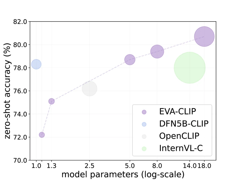
Figure 1 of EVA-CLIP-18B (arXiv:2402.04252), reproduced for editorial coverage.

EVA-CLIP-18B: scaling the recipe

Architecture. Vision encoder: 17.5B parameters across 48 layers, width 5120, 40 attention heads, patch size $14^2$, image resolution $224 \times 224$ (with $336 \times 336$ fine-tune) ⁶ . Text encoder: the EVA-02-CLIP-E/14+ text encoder reused without retraining, 695M parameters across 32 layers, width 1280, 20 attention heads. The asymmetry; vision encoder 25x larger than text encoder; is itself a finding: the paper argues the visual modality has more headroom to absorb scale at the current data scale.

Training procedure. LAMB optimiser ¹⁴ with $\beta_1 = 0.9$, $\beta_2 = 0.95$. Peak learning rates: $4 \times 10^{-4}$ vision, $4 \times 10^{-5}$ text. Batch size: 108k samples. Total samples seen: 6B. Training data: Merged-2B ^{12 13} . The recipe inherits FLIP-style image masking from Li et al. ¹⁴ , dropping a configurable fraction of image patches per step to recover forward-pass throughput. [Analysis] The headline efficiency claim of 80.7% average on 27 benchmarks with only 6B samples seen depends jointly on (a) EVA initialisation, (b) FLIP masking, and (c) LAMB optimisation. The paper does not isolate the contribution of each axis.

Initialisation from EVA. The image encoder is initialised from EVA-02 (a masked-image-modelling checkpoint that reconstructs CLIP features as targets) ⁷ . The recipe is therefore a two-stage training: stage 1 is masked-image modelling at smaller scale; stage 2 is contrastive language-image pretraining at 18B. This decomposes the data efficiency claim; most of the visual feature learning happens during stage 1 on ImageNet-22K plus the LAION subset used for EVA pretraining.

[Adapted] EVA-CLIP-18B’s contribution: scaling the EVA-CLIP-8B recipe to 18B with engineering optimisations (LAMB, FLIP masking, mixed precision, sharded data parallelism). No new loss or architectural innovation.

6. Mathematical contributions

The three papers share the cosine-similarity score $s_{ij} = \mathbf{x}_i \cdot \mathbf{y}_j$ (with both vectors $L_2$-normalised) and differ in how that score is converted into a loss.

MATH ENTRY 1: CLIP’s contrastive (InfoNCE) loss

• Source: CLIP Section 2.3 (paper provides pseudocode in Figure 3, equation form derivable from the pseudocode) ¹ .
• What it is: a symmetric softmax-cross-entropy loss that asks the model to score the diagonal of the $N \times N$ similarity matrix higher than the off-diagonal entries.
• Formal definition. Let $s_{ij} = \mathbf{x}_i \cdot \mathbf{y}_j$ and let $\tau$ be the learnable temperature. The image-to-text term is:

$\mathcal{L}_{i2t} = -\frac{1}{N} \sum_{i=1}^{N} \log \frac{\exp(s_{ii} / \tau)}{\sum_{j=1}^{N} \exp(s_{ij} / \tau)}$

The text-to-image term is the symmetric:

$\mathcal{L}_{t2i} = -\frac{1}{N} \sum_{j=1}^{N} \log \frac{\exp(s_{jj} / \tau)}{\sum_{i=1}^{N} \exp(s_{ij} / \tau)}$

The total loss is the average: $\mathcal{L}_{\text{CLIP}} = (\mathcal{L}_{i2t} + \mathcal{L}_{t2i}) / 2$.

• Each term explained and dimensional analysis.

  • $\mathbf{x}_i \in \mathbb{R}^d$ is the image embedding (e.g., $d = 512$). Already $L_2$-normalised, so $\lVert \mathbf{x}_i \rVert = 1$.
  • $\mathbf{y}_j \in \mathbb{R}^d$ is the text embedding, also $L_2$-normalised.
  • $s_{ij}$ is a scalar in $[-1, 1]$ because both vectors are unit-norm.
  • $\tau$ is a positive scalar; CLIP stores $\log \tau$ and clips $\log \tau \geq \log(1/100)$ so that $\tau \leq 100$.
  • The argument of the outer $\log$ is the categorical probability of the correct text being assigned to image $i$ under the softmax distribution over candidates.
  • The full loss is a scalar; its gradient flows through $\mathbf{x}_i, \mathbf{y}_j, \tau$.

• Worked numerical example. Take $N = 4$, $d = 4$. Suppose the four image embeddings and four text embeddings are (already $L_2$-normalised):

$$\mathbf{x}_1 = (1, 0, 0, 0), \quad \mathbf{x}_2 = (0, 1, 0, 0), \quad \mathbf{x}_3 = (0, 0, 1, 0), \quad \mathbf{x}_4 = (0, 0, 0, 1)$$ $$\mathbf{y}_1 = (0.9, 0.4, 0.1, 0.1), \quad \mathbf{y}_2 = (0.1, 0.9, 0.4, 0.1)$$ $$\mathbf{y}_3 = (0.1, 0.1, 0.9, 0.4), \quad \mathbf{y}_4 = (0.4, 0.1, 0.1, 0.9)$$

(Approximate normalisations; the numbers are illustrative.) Then $s_{11} = 0.9, s_{12} = 0.1, s_{13} = 0.1, s_{14} = 0.4$. Take $\tau = 0.07$ (CLIP’s initialisation). Then $s_{11}/\tau = 12.86$, $s_{12}/\tau = 1.43$, $s_{13}/\tau = 1.43$, $s_{14}/\tau = 5.71$. The softmax denominator for row 1 is $\exp(12.86) + \exp(1.43) + \exp(1.43) + \exp(5.71) \approx 384{,}000 + 4.18 + 4.18 + 302$. The probability of the correct text $\mathbf{y}_1$ is $\approx 384{,}000 / 384{,}310 \approx 0.999$, so $-\log(0.999) \approx 0.001$. The model already scores this example near-perfectly.

Now consider what happens with $\tau = 1$ (no temperature scaling): softmax denominator becomes $\exp(0.9) + \exp(0.1) + \exp(0.1) + \exp(0.4) \approx 2.46 + 1.11 + 1.11 + 1.49 = 6.17$, and the correct-class probability is $2.46 / 6.17 \approx 0.40$. Loss is $-\log(0.40) \approx 0.92$. The temperature matters enormously; it controls how sharply the loss differentiates between matching and non-matching pairs.

• Role: this is the single training objective driving CLIP’s encoders. Every parameter update flows from this loss.
• Edge cases: when $\tau \to 0$, the softmax becomes a hard argmax and gradients vanish for all but the highest-scoring candidate. CLIP’s clipping at $\tau \geq 1/100$ prevents this collapse. When $N = 1$ (single pair in a batch), the loss is identically zero because the softmax over one element is 1; the loss requires $N \geq 2$ to provide gradient signal.
• Novelty: [Adopted] from earlier contrastive multimodal work (ConVIRT) and InfoNCE (van den Oord et al. 2018). CLIP’s contribution is scale, not formulation.
• Transferability: [Analysis] reusable for any pair of modalities where (a) each instance has a natural counterpart in the other modality and (b) random pairs are mostly non-matching. Audio-text, video-text, point-cloud-text variants all use the same loss.
• Why it matters: the loss is what makes zero-shot transfer possible. By training to match against the full batch, the model learns embeddings that respect arbitrary class boundaries described by text rather than a fixed label set.

MATH ENTRY 2: SigLIP’s sigmoid loss

• Source: SigLIP Section 3, equation (1) ³ .
• What it is: a pairwise binary cross-entropy that treats each (image, text) pair in the batch as an independent positive-or-negative classification problem.
• Formal definition:

$\mathcal{L}_{\text{sigmoid}} = -\frac{1}{N} \sum_{i=1}^{N} \sum_{j=1}^{N} \log \sigma\left( z_{ij} \left( t \cdot \mathbf{x}_i \cdot \mathbf{y}_j + b \right) \right)$

where $z_{ij} = +1$ if $i = j$ (positive pair) and $z_{ij} = -1$ otherwise, $\sigma$ is the sigmoid function $\sigma(u) = 1 / (1 + e^{-u})$, $t$ is the learnable temperature (stored as $\log t$, initialised to $\log 10$), and $b$ is the learnable bias (initialised to $-10$) ³ .

• Each term explained and dimensional analysis.

  • $\mathbf{x}_i, \mathbf{y}_j$: same as MATH ENTRY 1; $L_2$-normalised embeddings in $\mathbb{R}^d$.
  • $\mathbf{x}_i \cdot \mathbf{y}_j$: scalar in $[-1, 1]$.
  • $t$: positive scalar; SigLIP scales similarities UP rather than dividing by $\tau$ as CLIP does. With $t = 10$, similarities of 0.9 become logits of 9.
  • $b$: scalar (typically large negative); shifts the decision boundary so the model can start with all-negative predictions.
  • $z_{ij}(t \mathbf{x}_i \cdot \mathbf{y}_j + b)$: scalar logit. For a positive pair with high similarity, the term is large positive; for a negative pair with high similarity, the term flips sign and becomes large negative, producing high loss.
  • The double sum is over all $N^2$ pairs, but each term is a constant-work scalar; the loss is $O(N^2)$ in pair computation and $O(1)$ in cross-worker communication for the loss itself (the similarity matrix still has to be assembled).

• Worked numerical example. Take $N = 3$, $t = 10$, $b = -10$. Suppose the diagonal similarities are $s_{11} = 0.9, s_{22} = 0.8, s_{33} = 0.7$ and the off-diagonal similarities are $s_{12} = 0.3, s_{13} = 0.2, s_{21} = 0.4, s_{23} = 0.1, s_{31} = 0.2, s_{32} = 0.3$. Then:

For positive pair $(1, 1)$: logit $= +1 \cdot (10 \cdot 0.9 + (-10)) = +1 \cdot (-1) = -1$. So $\sigma(-1) \approx 0.27$. Loss contribution: $-\log 0.27 \approx 1.31$. The model is currently SCORING the positive pair as more likely negative than positive; this is what the bias term at $b = -10$ is supposed to produce at initialisation so the model has a non-trivial gradient signal to learn from.

For negative pair $(1, 2)$: logit $= -1 \cdot (10 \cdot 0.3 + (-10)) = -1 \cdot (-7) = +7$. So $\sigma(7) \approx 0.999$. Loss contribution: $-\log 0.999 \approx 0.001$. The negative pair is already correctly classified.

After training, the diagonal similarities rise to e.g. $s_{11} \approx 0.99$; the positive logit becomes $+1 \cdot (10 \cdot 0.99 - 10) = -0.1$, $\sigma(-0.1) \approx 0.475$, loss $\approx 0.74$. With a higher learned $t$; say $t = 100$; the positive logit at $s_{11} = 0.99$ becomes $+1 \cdot (100 \cdot 0.99 + b)$; if $b$ has also moved (say to $-95$), the positive logit is $+1 \cdot (99 - 95) = +4$, $\sigma(4) \approx 0.982$, loss $\approx 0.018$. The learned $(t, b)$ pair encodes where the decision boundary sits in similarity space.

• Role: the SigLIP training objective. The structural advantage is that each $(i, j)$ term is independent; no row-wise or column-wise normalisation, no all-gather across workers.
• Edge cases: with $b = 0$ and small $t$, the loss collapses toward $-\log(0.5)$ for every pair at initialisation and the model has weak gradient signal to escape the equilibrium. SigLIP’s $b = -10$ initialisation breaks this. With $t \to \infty$, the loss approaches a hinge loss on the dot products.
• Novelty: [New]. The sigmoid loss for image-text pretraining at scale is the paper’s primary contribution. Related work on sigmoid contrastive loss in unimodal vision (Khosla et al. 2020 supervised contrastive) exists but did not apply at the CLIP scale.
• Transferability: [Analysis] the loss is directly applicable to any contrastive pretraining setting where global normalisation is expensive; distributed training across thousands of workers, federated training where gradients cannot be all-gathered, training under communication-bandwidth constraints. The sigmoid loss also opens the door to asynchronous training because the loss does not require a synchronous all-reduce.
• Why it matters: it decouples the loss formulation from batch size. CLIP needed batch size 32k because the InfoNCE loss requires enough negatives in the same batch to provide signal. SigLIP shows that the sigmoid loss reaches CLIP’s accuracy at batch 32k AND continues to improve modestly up to batch 256k AND retains most of its accuracy at batch sizes as small as 8k ³ .

MATH ENTRY 3: EVA-CLIP-18B’s training loss (inherited CLIP InfoNCE) with FLIP masking

• Source: EVA-CLIP-18B Section 3 plus inherited FLIP recipe ^{6 14} .
• What it is: the same InfoNCE loss as MATH ENTRY 1, applied to image embeddings computed from a fraction $1 - r$ of image patches, where $r$ is the FLIP mask ratio.
• Formal definition: identical to MATH ENTRY 1, with $f_\theta(I) = \text{ViT}(\text{drop}(I, r))$, i.e., a stochastic patch-dropping operation is applied before the ViT forward pass.
• Each term explained: FLIP masking ratio $r$ is typically 0.5 (drop 50% of patches), reducing the ViT’s forward FLOPs by approximately $(1 - r)^2$ in the attention block and by $(1 - r)$ in the feed-forward block. Effective speedup is roughly 2x at $r = 0.5$, paid for by a small accuracy loss that can be recovered with a short unmasked fine-tune.
• Worked example: at $r = 0.5$ on a 224x224 image with 14x14 patches, the ViT processes 98 patches per image instead of 196. For a ViT-18B vision encoder, this halves the attention complexity from $\sim 196^2 \cdot d$ to $\sim 98^2 \cdot d$ per layer, freeing compute that the paper redirects toward larger batch sizes.
• Role: enables the 6B-samples-seen budget to cover an 18B encoder.
• Edge cases: aggressive masking ($r \geq 0.75$) degrades downstream accuracy substantially; the paper uses $r = 0.5$ as the operating point.
• Novelty: [Adopted] from FLIP (Li et al. 2023, CVPR 2023) ¹⁴ .
• Transferability: [Analysis] applicable to any image-text training run constrained by ViT forward-pass compute.
• Why it matters: it is the engineering trick that makes 18B-parameter training tractable on Merged-2B within the paper’s compute budget.

[Analysis] Comparison of the three formulations. CLIP’s loss requires global normalisation across the batch; communication cost scales with $N$. SigLIP’s loss does not; communication cost is independent of how the loss is computed (the similarity matrix still requires the all-gather of embeddings, but the loss arithmetic itself is local). EVA-CLIP-18B uses CLIP’s loss but reduces forward-pass cost via FLIP masking. The three papers thus attack different engineering bottlenecks; loss formulation (SigLIP), forward-pass compute (EVA-CLIP-18B), and the original scale demonstration (CLIP).

7. Algorithmic contributions

ALGORITHM ENTRY 1: CLIP training step (the headline algorithm reproduced in CLIP Figure 3 pseudocode) ¹ .

• Source: CLIP Figure 3 pseudocode.
• Purpose: one gradient step of contrastive image-text pretraining.
• Inputs:
  • image_batch: tensor of shape $(N, 3, H, W)$; N RGB images of size $H \times W$ (CLIP: $224 \times 224$).
  • text_batch: tensor of shape $(N, L)$; N token sequences of length $L$ (CLIP: $L = 76$).
  • image_encoder, text_encoder: trainable modules.
  • W_i, W_t: linear projection matrices into the shared embedding space $\mathbb{R}^d$.
  • tau: learnable temperature scalar (stored as $\log \tau$).
• Outputs: scalar loss; gradients applied to all trainable parameters.
• Pseudocode (faithful reconstruction from CLIP Figure 3):

# CLIP training step (per Radford et al. 2021, Figure 3)
def clip_train_step(image_batch, text_batch,
                    image_encoder, text_encoder,
                    W_i, W_t, log_tau):
    # 1. Encode each modality to its native dim
    I_f = image_encoder(image_batch)        # (N, d_i)
    T_f = text_encoder(text_batch)          # (N, d_t)

    # 2. Project into shared embedding space
    I_e = l2_normalize(I_f @ W_i, axis=1)   # (N, d)
    T_e = l2_normalize(T_f @ W_t, axis=1)   # (N, d)

    # 3. Compute similarity matrix scaled by temperature
    tau = exp(log_tau)                       # clipped so tau <= 100
    logits = (I_e @ T_e.T) / tau             # (N, N)

    # 4. Symmetric cross-entropy against diagonal targets
    labels = arange(N)
    loss_i = cross_entropy(logits, labels)         # image -> text
    loss_t = cross_entropy(logits.T, labels)       # text -> image
    loss = (loss_i + loss_t) / 2

    return loss

• Hand-traced example. Take $N = 2$, $d = 4$. Suppose after encoding and projection:
  • $I_e[0] = (1, 0, 0, 0)$, $I_e[1] = (0, 1, 0, 0)$
  • $T_e[0] = (0.8, 0.6, 0, 0)$, $T_e[1] = (0.1, 0.9, 0.4, 0)$ (post-$L_2$-normalisation values rounded)
  • $\log \tau = -2.66$ (so $\tau \approx 0.07$).

Step 3: logits[0][0] $= (1 \cdot 0.8 + 0 + 0 + 0) / 0.07 \approx 11.4$. logits[0][1] $= (1 \cdot 0.1 + 0 + 0 + 0) / 0.07 \approx 1.4$. logits[1][0] $= (0 + 1 \cdot 0.6 + 0 + 0) / 0.07 \approx 8.6$. logits[1][1] $= (0 + 1 \cdot 0.9 + 0 + 0) / 0.07 \approx 12.9$.

Step 4 image-to-text: row 0 softmax $\propto (e^{11.4}, e^{1.4}) \approx (89{,}321, 4.06)$. P(correct) $\approx 0.99996$. $-\log P \approx 4 \times 10^{-5}$.

Row 1 softmax $\propto (e^{8.6}, e^{12.9}) \approx (5{,}432, 400{,}312)$. P(correct = column 1) $\approx 0.9866$. $-\log P \approx 0.0135$.

Text-to-image (column softmax): identical structure by symmetry of the example. Final loss $\approx (4 \times 10^{-5} + 0.0135 + \text{column terms}) / 4$.

Variable state at end of step: loss is a scalar tensor connected to the computational graph; loss.backward() populates gradients on image_encoder, text_encoder, W_i, W_t, log_tau.

• Complexity: forward $O(N \cdot C_{\text{enc}} + N^2 d)$ where $C_{\text{enc}}$ is the per-sample encoder cost; communication $O(N d)$ for all-gather of embeddings; backward $O(N \cdot C_{\text{enc}})$. Bottleneck step: the encoder forward pass dominates at CLIP’s batch size of 32,768.
• Hyperparameters: batch size $N = 32{,}768$, learning rate (peak $5 \times 10^{-4}$ for ViT-L/14), Adam $\beta_1 = 0.9, \beta_2 = 0.98$, weight decay 0.2, cosine schedule, 32 training epochs over WIT (so 32 × 400M / 32k $\approx$ 400k steps) ² .
• Failure modes: at very small batches ($N \leq 512$), the contrastive signal weakens because fewer negatives are available per row; loss converges to a poor optimum.
• Novelty: [Adopted] formulation; [New] application at 400M-pair scale.
• Transferability: [Analysis] this pseudocode is the de-facto template for any contrastive image-text training run; OpenCLIP, EVA-CLIP, and SigLIP’s reference implementations all derive from it.

ALGORITHM ENTRY 2: SigLIP training step (sigmoid loss, no all-gather on the loss) ³ .

• Source: SigLIP Section 3 pseudocode, reconstructed faithfully.
• Purpose: one gradient step of pairwise-sigmoid image-text pretraining.
• Inputs: same as ALGORITHM ENTRY 1, plus learnable bias b.
• Outputs: scalar loss; gradients on all trainable parameters.
• Pseudocode (faithful reconstruction):

# SigLIP training step (per Zhai et al. 2023, Section 3)
def siglip_train_step(image_batch, text_batch,
                      image_encoder, text_encoder,
                      log_t, b):
    I_e = l2_normalize(image_encoder(image_batch), axis=1)   # (N, d)
    T_e = l2_normalize(text_encoder(text_batch), axis=1)     # (N, d)

    t = exp(log_t)                          # initialised log(10)
    logits = t * (I_e @ T_e.T) + b          # (N, N); b is scalar

    # Construct z_ij: +1 on diagonal, -1 off-diagonal
    labels = 2 * eye(N) - ones((N, N))      # (N, N), values in {-1, +1}

    # Pairwise sigmoid cross-entropy
    loss = -mean(log_sigmoid(labels * logits))

    return loss

• Hand-traced example. Take $N = 3$, $\log t = \log 10$ (so $t = 10$), $b = -10$, and the similarity matrix from the worked example in MATH ENTRY 2:

logits matrix becomes:

	$j=1$	$j=2$	$j=3$
$i=1$	$10 \cdot 0.9 - 10 = -1$	$10 \cdot 0.3 - 10 = -7$	$10 \cdot 0.2 - 10 = -8$
$i=2$	$10 \cdot 0.4 - 10 = -6$	$10 \cdot 0.8 - 10 = -2$	$10 \cdot 0.1 - 10 = -9$
$i=3$	$10 \cdot 0.2 - 10 = -8$	$10 \cdot 0.3 - 10 = -7$	$10 \cdot 0.7 - 10 = -3$

labels matrix:

	$j=1$	$j=2$	$j=3$
$i=1$	$+1$	$-1$	$-1$
$i=2$	$-1$	$+1$	$-1$
$i=3$	$-1$	$-1$	$+1$

Element-wise labels * logits:

	$j=1$	$j=2$	$j=3$
$i=1$	$-1$	$+7$	$+8$
$i=2$	$+6$	$-2$	$+9$
$i=3$	$+8$	$+7$	$-3$

log_sigmoid of each entry (recall $\log \sigma(u) = -\log(1 + e^{-u})$): negative-valued entries on the diagonal where the positive pairs are under-scored, and near-zero values on the off-diagonal where the negatives are correctly classified. Sum and negate: $-\text{mean}(\log \sigma)$ produces a scalar loss roughly in the range $[0.5, 1.5]$ at initialisation.

Variable state at end: gradients flow through $\mathbf{x}_i, \mathbf{y}_j, t, b$ to update the encoders, the temperature, and the bias.

• Complexity: forward $O(N \cdot C_{\text{enc}} + N^2 d)$, the same as CLIP; the saving is in the loss step itself (no row-softmax, hence no per-row reduction). On distributed training, the embeddings still need to be all-gathered to build the $N \times N$ similarity matrix, but each worker can compute its own portion of the loss without the cross-row dependency.
• Hyperparameters: $\log t$ initialised to $\log 10$, $b$ initialised to $-10$, Adafactor optimiser, learning rate $10^{-3}$ (SigLIP B/16), weight decay $10^{-4}$.
• Failure modes: collapse if $b$ is initialised too close to 0 (positive-pair probability $\approx 0.5$ at start, vanishing gradient); collapse if $t$ is initialised very large (saturates sigmoid).
• Novelty: [New]. The loss formulation, plus the chunked-mask variant that lets workers exchange only partial similarity sub-matrices.
• Transferability: [Analysis] same applicability as MATH ENTRY 2; works for any contrastive setting where global softmax is expensive.

ALGORITHM ENTRY 3: EVA-CLIP-18B FLIP-style masking pass (training step inherits CLIP’s loss; the algorithmic novelty is in the forward pass) ^{6 14} .

• Source: EVA-CLIP-18B Section 3 and inherited FLIP Section 3.
• Purpose: drop a fraction $r$ of image patches before the ViT forward pass to recover throughput.
• Inputs: image_batch shape $(N, 3, H, W)$; patch grid $(H/p) \times (W/p)$ for patch size $p$; mask ratio $r$.
• Outputs: image embeddings $\mathbf{x}_i$ for the contrastive loss.
• Pseudocode (faithful reconstruction):

# EVA-CLIP-18B image branch with FLIP masking
def vit_with_flip_mask(image_batch, vit, r=0.5):
    patches = patchify(image_batch)             # (N, P, p*p*3); P = (H/p)*(W/p)
    P = patches.shape[1]
    keep = int(P * (1 - r))

    # Random per-sample mask: keep `keep` patches uniformly at random
    perm = random_permutation(N, P)
    kept_patches = gather(patches, perm[:, :keep])  # (N, keep, p*p*3)

    # ViT forward only on kept patches (plus class token)
    x = vit(kept_patches)                        # (N, d)

    return l2_normalize(x, axis=1)

• Hand-traced example. Take $H = W = 224$, $p = 14$, so $P = 16 \times 16 = 256$ patches. With $r = 0.5$, keep $= 128$. For a single image, suppose perm[0] puts patches $\{3, 17, 42, ..., 251\}$ in the first 128 positions. The ViT receives a (1, 128, 588)-shaped tensor (each patch flattened to $14 \times 14 \times 3 = 588$ values). Forward pass complexity drops from $O(256^2 \cdot d) = O(65{,}536 d)$ per attention layer to $O(128^2 \cdot d) = O(16{,}384 d)$; a 4x reduction in attention cost.
• Complexity: forward FLOPs reduce by $\sim (1-r)^2$ in attention and $\sim (1-r)$ in feed-forward. At $r = 0.5$, effective ViT throughput roughly doubles.
• Hyperparameters: $r = 0.5$ in EVA-CLIP-18B’s main run; some baselines used $r = 0$ (unmasked) to verify the masking does not contribute most of the headline accuracy.
• Failure modes: at $r \geq 0.75$, downstream accuracy drops substantially; the paper recommends $r \leq 0.5$ for the contrastive run, plus an optional short unmasked fine-tune for the final percent of accuracy.
• Novelty: [Adopted] from FLIP.
• Transferability: [Analysis] applicable to any ViT-based pretraining run constrained by forward-pass compute.

8. Specialised design contributions

8A. LLM / prompt design

Not applicable to this paper cluster. The three works pretrain vision-language encoders; no LLM is used in the training loop. CLIP introduced prompt templates (“a photo of a {class}”) at inference for zero-shot classification, but this is a downstream-usage pattern rather than a method component.

8B. Architecture-specific details

• CLIP attention. Standard pre-norm Transformer for both image and text encoders ² . The text encoder uses causal masking; the image encoder is bidirectional within the patch sequence.
• SigLIP architecture. Uses the So400m (“Shape-Optimised 400M”) ViT variant ³ , a re-shaped ViT family designed to maximise compute-efficiency at the 400M-parameter scale. Patch size 16x16, image resolution 224 or 384.
• EVA-CLIP-18B architecture. ViT-18B with 48 layers, width 5120, MLP ratio 4 (so MLP dim 20480), 40 attention heads, head dim 128, patch size 14x14, image resolution 224 ⁶ . Uses RoPE (rotary position embeddings) and SwiGLU activations inherited from EVA-02. Text encoder kept at EVA-02-CLIP-E/14+‘s 695M parameters (32 layers, width 1280, 20 heads).

8C. Training specifics

• CLIP compute. ViT-L/14 took 12 days on 256 NVIDIA V100 GPUs ² . RN50x64 took 18 days on 592 V100s. Mixed precision throughout.
• SigLIP compute. ViT-B/16 SigLIP trained on TPUv4 pods; the “84.5% ImageNet zero-shot in two days on four TPUv4 chips” claim refers specifically to the LiT (Locked-image Tuning) variant where the image encoder is frozen ³ .
• EVA-CLIP-18B compute. Trained on a mix of NVIDIA A100 and H100 nodes; the paper does not give a precise GPU-day number but states 6B samples seen at batch 108k, so $\sim$56k optimisation steps. [Analysis] Order-of-magnitude estimate: at $\sim$2 trillion FLOPs per forward-backward pass for the 18B ViT and 6B samples processed, total training compute is on the order of $10^{22}$ FLOPs, consistent with a multi-thousand-GPU run for several weeks.

8D. Inference / deployment specifics

All three encoders support standard cosine-similarity zero-shot classification. EVA-CLIP-18B is too large for typical single-GPU deployment; the released checkpoint requires tensor-parallel inference for full-precision use. SigLIP B/16 and L/16 ship as drop-in replacements in standard CLIP-API libraries (HuggingFace Transformers, OpenCLIP), and SigLIP 2 ships pre-baked tokenisers for multilingual text ⁵ .

9. Experiments and results

Datasets. CLIP evaluated on 27 zero-shot classification benchmarks plus ImageNet-1K and its robustness variants (ImageNet-V2, ImageNet-A, ImageNet-R, ImageNet-Sketch, ObjectNet) ² . SigLIP evaluated on the same 27-task suite plus retrieval benchmarks (COCO, Flickr30K) ³ . EVA-CLIP-18B evaluated on the same 27-task suite plus the LVIS detection and ADE20K segmentation transfer tasks ⁶ .

Baselines. CLIP’s baselines are supervised ImageNet pretraining (ResNet-50, ResNet-101) and earlier vision-language work (ConVIRT, VirTex, ICMLM). SigLIP’s baselines are CLIP and LiT. EVA-CLIP-18B’s baselines are OpenCLIP-G/14, EVA-02-CLIP-E/14+, EVA-CLIP-8B, and InternVL-C.

Evaluation metrics. Zero-shot top-1 ImageNet accuracy is the headline number for all three papers. Secondary metrics: 27-benchmark average (EVA-CLIP-18B), COCO image-text retrieval R@1 (SigLIP), and robustness deltas on ImageNet variants (CLIP).

Key result table (reproduced inline with attribution).

Model	Params (vision)	Pretrain data	Samples seen	ImageNet zero-shot top-1
CLIP ViT-L/14	304M	WIT 400M	12.8B (32 epochs)	75.5% (paper: 76.2% at $336^2$ 2 )
OpenCLIP ViT-G/14	1.0B	LAION-2B	39B	80.1% 8
SigLIP So400m/14	400M	WebLI	40B (paper)	83.1% 3
EVA-02-CLIP-E/14+	4.4B	LAION-2B + COYO	9B	82.0% 7
EVA-CLIP-8B	7.5B	Merged-2B	9B	83.5% 6
EVA-CLIP-18B	17.5B	Merged-2B	6B	83.8% 6

Reproduced from CLIP Table 9 (arXiv:2103.00020), SigLIP Table 1 (arXiv:2303.15343), and EVA-CLIP-18B Table 2 (arXiv:2402.04252), for editorial coverage.

Figure 2 of EVA-CLIP-18B (arXiv:2402.04252), reproduced for editorial coverage.

Main quantitative results.

• CLIP: ViT-L/14 reaches 75.5% ImageNet zero-shot top-1 and 76.2% at $336 \times 336$ fine-tune resolution ² . Across the 27-task suite, CLIP averages above all prior zero-shot methods at the time of publication.
• SigLIP: So400m/14 reaches 83.1% ImageNet zero-shot top-1, exceeding all prior CLIP-line models at comparable parameter counts ³ . The paper’s batch-size sweep shows the sigmoid loss matches softmax InfoNCE at batch 32k and modestly exceeds it at batches up to 256k.
• EVA-CLIP-18B: 80.7% average across 27 benchmarks; 83.8% on ImageNet-1K zero-shot ⁶ .

Supplementary results. SigLIP’s appendix includes a small-batch sweep showing the sigmoid loss retains $\sim$71% ImageNet accuracy at batch 8k, where the softmax InfoNCE drops to $\sim$66% ³ . EVA-CLIP-18B’s appendix reports robustness deltas on ImageNet-V2 (+1.3 points over EVA-CLIP-8B), ImageNet-R (+1.1), ImageNet-A (+2.5), and ObjectNet (+1.2) ⁶ .

Ablations.

• CLIP ablations: prompt engineering (+1.3 points on ImageNet zero-shot), prompt ensembling (+0.5), encoder architecture (ViT vs ResNet at matched compute; ViT consistently wins), dataset scale (linear scaling with log of dataset size to about 400M) ² .
• SigLIP ablations: batch size sweep, $t$ and $b$ initialisation sweep, optimizer choice (Adafactor vs Adam; Adafactor is more memory-efficient at large batch but otherwise equivalent) ³ .
• EVA-CLIP-18B ablations: scaling from EVA-CLIP-8B to 18B yields +0.3 points on ImageNet zero-shot; a small headline gain that the paper frames as evidence that the recipe is approaching diminishing returns at this scale ⁶ .

Figure 3 of EVA-CLIP-18B (arXiv:2402.04252), reproduced for editorial coverage.

Hyperparameter sensitivity.

• CLIP: $\tau$ initialisation and clipping are load-bearing (untested but emphasised by the authors as critical).
• SigLIP: $b$ initialisation matters more than $t$; the bias controls early-training calibration. Untested initialisations diverge during the first 1000 steps.
• EVA-CLIP-18B: LAMB’s $\beta_2$ matters more than learning rate. $\beta_2 = 0.95$ outperforms $\beta_2 = 0.999$ at this scale.

Independent benchmark cross-checks. OpenCLIP’s reproduction of the CLIP recipe ⁸ validates the original CLIP zero-shot ImageNet numbers and shows that LAION-2B (open data) reaches similar accuracy as CLIP’s closed WIT at matched compute. Papers With Code’s zero-shot ImageNet leaderboard ¹⁵ ranks EVA-CLIP-18B and SigLIP So400m/14 near the top of the open-weights category as of late 2025. [Analysis] The SOTA picture is fragmented across reporting protocols (224 vs 336 resolution, prompt-template choice, ensemble vs single prompt). The 80.7% / 83.8% EVA-CLIP-18B numbers are the paper’s framing; independent third-party reproduction of the 18B model has not yet been published as of 2026-05-19 owing to its scale.

Evidence audit. [Analysis]

• Strongly supported: the contrastive image-text recipe scales with data and parameters (CLIP, OpenCLIP, EVA-CLIP-18B all confirm this); the sigmoid loss matches softmax InfoNCE at standard batch sizes (SigLIP’s main result, independently reproduced by HuggingFace’s SigLIP implementation).
• Partially supported: the sigmoid loss exceeds softmax at very small batch sizes (SigLIP shows this in their ablation, but limited independent replication).
• Narrow evidence: EVA-CLIP-18B’s claim that scaling to 18B yields meaningful gains over 8B; the +0.3-point gain on ImageNet is small relative to within-run variance, and the paper does not provide enough runs to estimate variance.

10. Technical novelty summary

Component	Type	Novelty level	Justification	Source
Contrastive image-text loss at 400M scale	CLIP	Combination novel	The loss formulation was adopted, the scale was new	CLIP Section 2
Zero-shot prompt-based classification	CLIP	Incrementally novel	Prompts existed for language models; CLIP applied them to vision	CLIP Section 3
Pairwise sigmoid loss for V-L pretraining	SigLIP	Fully novel	The first paper to apply sigmoid contrastive loss at CLIP scale	SigLIP Section 3
$b$ bias term for sigmoid calibration	SigLIP	Fully novel	New, paper-specific contribution	SigLIP Section 3.2
EVA initialisation (MIM → CLIP)	EVA series	Combination novel	MIM pretraining was known; using it to initialise CLIP at scale was new	EVA Section 3
FLIP masking inside CLIP training	EVA-CLIP-18B	Adopted	From FLIP (Li et al. 2023)	EVA-CLIP-18B Section 3
LAMB at 18B contrastive scale	EVA-CLIP-18B	Incrementally novel	LAMB existed; applying it to 18B V-L pretraining was new	EVA-CLIP-18B Section 3
27-benchmark zero-shot averaging	EVA-CLIP-18B	Adopted	Evaluation protocol from OpenCLIP	OpenCLIP Section 5

Single most novel contribution. The sigmoid loss formulation in SigLIP; equation (1) of the paper; is the single most novel mathematical contribution across the three works. CLIP scaled an existing loss; EVA-CLIP-18B scaled an existing recipe. SigLIP changed the loss itself, and the change has direct consequences for distributed training, batch-size flexibility, and downstream-model design.

What the papers do NOT claim to be novel.

• CLIP does not claim the InfoNCE loss as novel; credits van den Oord et al. (2018) and ConVIRT.
• SigLIP does not claim ViT or the text Transformer as novel.
• EVA-CLIP-18B does not claim FLIP masking, LAMB, or the EVA architecture as novel.

11. Situating the work

The prior-art landscape these papers respond to:

• Supervised pretraining (ResNet, ViT); the recipe CLIP displaced.
• Unimodal contrastive learning (SimCLR, MoCo); the loss family CLIP borrowed from.
• Captioning-based vision-language pretraining (CoCa, BLIP); the captioning alternative to contrastive.
• Masked image modelling (MAE, EVA); the self-supervised alternative that EVA-CLIP-18B blends with the contrastive recipe.
• Open-source reproductions (OpenCLIP); the line that validated CLIP on public data.

Contemporaneous related work.

• Beyer et al. (2024), PaliGemma. Built directly on top of SigLIP encoders; the SigLIP authors’ team at Google argued that the sigmoid loss’s per-pair independence makes downstream VLM training cleaner because the encoder’s frozen embeddings don’t depend on the batch composition. [External comparison] This citation is the strongest evidence that SigLIP’s loss has practical downstream consequences beyond benchmark numbers.
• Cherti et al. (2023), OpenCLIP. Established that LAION-2B + EVA-style training matches CLIP-on-WIT at comparable compute ⁸ . EVA-CLIP-18B builds directly on this lineage. The specific technical relationship: OpenCLIP demonstrated open-data parity at $\sim$1B vision parameters; EVA-CLIP-18B extended the demonstration to 18B vision parameters using the same data lineage plus EVA initialisation and FLIP masking.
• Tschannen et al. (2025), SigLIP 2. Adds captioning, self-distillation, masked prediction, and online data curation on top of SigLIP 1’s sigmoid loss ⁵ . The specific technical relationship: SigLIP 2 keeps the sigmoid loss verbatim and stacks complementary objectives, suggesting the loss formulation has matured into a stable foundation.

[Reviewer Perspective] Strongest skeptical objection. The headline gains in EVA-CLIP-18B are small relative to the 2x scale jump (8B to 18B). The 80.7% average on the 27-benchmark suite is +0.7 points over EVA-CLIP-8B’s reported number on the same suite. The scaling-law slope is flattening, and at 18B vision parameters the recipe may be approaching the data-side ceiling of Merged-2B. A skeptical reviewer would ask: is the right next step more parameters, more data, or a different objective?

[Reviewer Perspective] Strongest author-side rebuttal. The 80.7% number is an average over 27 benchmarks; on the harder benchmarks (ImageNet-A, ObjectNet, ImageNet-Sketch), the gains over 8B are 2-3 points each. The recipe is paying off where the supervised baselines struggle most; robustness, distribution shift, fine-grained tasks.

What remains unsolved. None of the three papers explains why the contrastive loss produces representations that transfer to localisation tasks (detection, segmentation) less well than masked-image pretraining does. SigLIP 2’s addition of dense-prediction-friendly objectives is an empirical fix; the underlying question of why CLIP’s representations are biased toward global semantics rather than local features remains open.

Three future research directions.

• Asynchronous SigLIP at federated scale. [Analysis] The sigmoid loss’s per-pair independence makes it the natural starting point for federated or asynchronous training where global all-gathers are infeasible. No published paper has attempted this as of 2026-05-19.
• EVA-style initialisation for SigLIP. [Analysis] EVA-CLIP-18B initialises from EVA-02 (MIM) and then trains with CLIP’s softmax InfoNCE loss. The combination of EVA initialisation with SigLIP’s loss has not been published; the cross-recipe ablation would isolate the contribution of initialisation versus loss formulation.
• Loss-function geometry at 100B+ parameters. [Reviewer Perspective] At what point does the choice of loss formulation matter less than the choice of initialisation, data composition, and optimizer? EVA-CLIP-18B suggests the loss matters less than initialisation at 18B; whether this holds at 100B+ is open.

12. Critical analysis

Strengths with concrete evidence.

• CLIP’s zero-shot ImageNet of 75.5% (76.2% at higher resolution) without any ImageNet-1K labels in training is reproducible and has been independently verified by OpenCLIP ⁸ .
• SigLIP’s batch-size flexibility is demonstrated by a full sweep from batch 8k to batch 256k in the paper’s main experiments ³ , with reproducible code released ¹⁰ .
• EVA-CLIP-18B’s 80.7% average is supported by a per-benchmark table covering all 27 tasks ⁶ .

Weaknesses explicitly stated by the authors.

• CLIP: the paper acknowledges that the WIT dataset is not released, limiting reproducibility; that the recipe inherits the social biases of web-scraped data; that downstream task accuracy on fine-grained categories (CLIP Section 5) underperforms supervised baselines ² .
• SigLIP: limited gains over softmax InfoNCE at very large batches (the sigmoid advantage is concentrated at small and moderate batch sizes); the bias term $b$ requires careful initialisation ³ .
• EVA-CLIP-18B: training cost limits the number of full runs the authors could perform, so variance estimates are absent; the paper acknowledges that the 80.7% average’s variance across runs is not reported ⁶ .

Weaknesses not stated or understated. [Reviewer Perspective]

• CLIP’s lack of localised features is a real limitation for downstream detection / segmentation tasks; DINOv2 and SigLIP 2 both target this gap directly.
• SigLIP’s headline “84.5% in two days on four TPUv4 chips” is a LiT result (image encoder frozen from a strong supervised checkpoint); the comparison to CLIP at this number is not apples-to-apples because CLIP trains the image encoder from scratch.
• EVA-CLIP-18B’s +0.3-point gain on ImageNet over EVA-CLIP-8B is within likely run-to-run variance for the recipe; the paper would have benefited from at least one full re-run to quantify confidence.

Reproducibility check.

• Code: released for all three. CLIP ($\to$ github.com/openai/CLIP ⁹ ), SigLIP ($\to$ github.com/google-research/big_vision ¹⁰ ), EVA-CLIP-18B ($\to$ github.com/baaivision/EVA ¹¹ ).
• Data: CLIP’s WIT not released. SigLIP’s WebLI not released. EVA-CLIP-18B’s Merged-2B IS publicly available (LAION-2B ¹² + COYO-700M ¹³ ).
• Hyperparameters: fully disclosed for all three.
• Compute: CLIP and EVA-CLIP-18B report compute; SigLIP reports TPUv4 chip-days for the LiT variant only.
• Trained model weights: CLIP releases ViT-B/32 and ViT-L/14 weights (no ResNet-50x64); SigLIP releases all variants via HuggingFace; EVA-CLIP-18B releases the full 18B checkpoint.
• Evaluation set: all three use public benchmarks; eval pipelines are open.
• Overall: partially reproducible for CLIP and SigLIP (data closed); fully reproducible for EVA-CLIP-18B (all components public, subject to access to thousand-GPU-class compute).

Methodology

• Sample size: CLIP; 400M image-text pairs, 32 epochs (12.8B samples seen). SigLIP; WebLI, 40B samples seen (paper main runs). EVA-CLIP-18B; Merged-2B (~2.0B unique pairs), 6B samples seen (~3 effective epochs).
• Evaluation set: 27 zero-shot classification benchmarks shared across all three, with ImageNet-1K as headline. Robustness variants (ImageNet-V2/R/A/Sketch, ObjectNet) covered in CLIP and EVA-CLIP-18B; SigLIP additionally covers COCO retrieval.
• Baselines: CLIP; supervised ResNet, ConVIRT, VirTex. SigLIP; CLIP, LiT. EVA-CLIP-18B; OpenCLIP-G/14, EVA-02-CLIP-E/14+, EVA-CLIP-8B, InternVL-C.
• Hardware/compute: CLIP; 256 V100 (ViT-L/14, 12 days), 592 V100 (RN50x64, 18 days). SigLIP; TPUv4 pods (precise chip-day count given only for LiT result). EVA-CLIP-18B; multi-thousand GPU mix of A100 / H100; precise compute budget not reported in the paper.

Generalisability. The contrastive image-text recipe transfers cleanly to other domains: audio-text (CLAP), video-text (VideoCLIP, InternVideo), point-cloud-text (PointCLIP). The sigmoid loss has been adopted in those follow-ups as well. The EVA initialisation strategy is specific to the vision domain because it requires a strong masked-image-modelling teacher; it does not transfer directly to text-only or audio-only pretraining.

Assumption audit. Revisiting Section 3 assumptions: the cosine-geometry assumption is empirically validated across all three papers; the random-pairs-are-mostly-non-matching assumption holds at web scale but is fragile in domain-specific corpora (medical imaging, satellite imagery), where many image-text pairs may share semantic content. [Analysis] Researchers fine-tuning CLIP-line encoders on specialised corpora should expect the contrastive signal to weaken and may need to switch to a hard-negative-mining variant.

What would make the papers significantly stronger. [Analysis]

• CLIP: a public release of WIT (or at least a sample) would close the reproducibility gap.
• SigLIP: ablations isolating the contribution of $b$ versus $t$ separately, and a derivation showing why $b = -10$ specifically is the right initialisation.
• EVA-CLIP-18B: variance estimates from at least one additional full training run at 18B scale to confirm the +0.3-point ImageNet gain over 8B is not within-run noise.

13. What is reusable for a new study

REUSABLE COMPONENT 1: The contrastive image-text training step (ALGORITHM ENTRY 1).

• What it is: the basic CLIP training-step pseudocode.
• Why worth reusing: the de-facto template for any contrastive multimodal pretraining run.
• Preconditions: sufficient batch size ($\geq$ 8k) and a paired dataset of at least 100M instances.
• What would need to change in a different setting: the encoders ($\text{ViT}, \text{Transformer}$) can be swapped for any modality-specific architecture; the loss is modality-agnostic.
• Risks: collapse at small batch sizes; sensitive to temperature initialisation.
• Interaction effects: dataset quality matters more than recipe details below the $\sim$100M-pair threshold.

REUSABLE COMPONENT 2: SigLIP’s sigmoid loss (MATH ENTRY 2 / ALGORITHM ENTRY 2).

• What it is: the pairwise sigmoid loss formulation.
• Why worth reusing: removes the global-batch normalisation requirement of softmax InfoNCE; works at small AND large batch sizes; clean to implement in distributed training.
• Preconditions: $L_2$-normalised embeddings; learnable temperature $t$ and bias $b$ both initialised carefully.
• What would need to change: not modality-specific; works for any contrastive setting.
• Risks: collapse if $b$ is initialised too close to 0; saturation if $t$ is initialised too large.
• Interaction effects: pairs naturally with chunked / asynchronous distributed training schemes.

REUSABLE COMPONENT 3: EVA initialisation (MIM-pretrained encoder as the starting point for contrastive training).

• What it is: a two-stage recipe; stage 1 is masked-image modelling at smaller scale; stage 2 is contrastive language-image pretraining initialised from the stage-1 encoder.
• Why worth reusing: data efficiency. The 6B-samples-seen budget for EVA-CLIP-18B’s stage 2 is small compared to OpenCLIP’s 39B-samples budget for a 1B-parameter model.
• Preconditions: a strong MIM checkpoint at the target encoder size.
• What would need to change in a different setting: stage 1 needs to be redone for each new encoder size; not a free swap.
• Risks: stage 1 takes substantial compute; the two-stage recipe is more complex than single-stage CLIP-style training.
• Interaction effects: pairs naturally with FLIP masking in stage 2 because the MIM checkpoint is already accustomed to masked inputs.

REUSABLE COMPONENT 4: FLIP masking inside the contrastive forward pass (ALGORITHM ENTRY 3).

• What it is: a fixed-fraction random patch drop applied before the ViT forward pass during contrastive training.
• Why worth reusing: roughly 2x ViT forward-pass throughput at $r = 0.5$ with minimal accuracy cost.
• Preconditions: a ViT-class image encoder; appropriate compensation in the loss scaling.
• What would need to change: mask ratio $r$ should be tuned for the target encoder size; smaller encoders tolerate less masking.
• Risks: aggressive masking ($r \geq 0.75$) degrades downstream accuracy; the recipe needs a short unmasked fine-tune for the final accuracy points.
• Interaction effects: composes well with EVA initialisation because the stage-1 MIM model has already learned to process masked patches.

Dependency map. The four reusable components form a stack: COMPONENT 1 (the basic training step) is the foundation; COMPONENT 2 (sigmoid loss) is a swap-in replacement for the loss inside COMPONENT 1; COMPONENT 3 (EVA initialisation) provides the starting weights for the encoders in COMPONENT 1; COMPONENT 4 (FLIP masking) is an additive efficiency improvement to the forward pass of COMPONENT 1.

Recommendation. [Analysis] For a research group building a new contrastive multimodal model from scratch, the highest-value reusable components are: (a) COMPONENT 2; adopt the sigmoid loss to decouple training from batch size and simplify distributed scheduling; (b) COMPONENT 3; if the target encoder is $\geq$ 1B parameters, the EVA-style two-stage recipe is the most compute-efficient path; (c) COMPONENT 4; adopt FLIP masking at $r = 0.5$ as a default efficiency trick when ViT forward-pass cost dominates.

[Analysis] Studies most likely to benefit: federated / asynchronous training of vision-language encoders, dense-prediction-friendly multimodal pretraining, and domain-specific contrastive pretraining on smaller corpora where the global-batch InfoNCE objective is impractical.

14. Known limitations and open problems

Limitations explicitly stated by the authors.

• CLIP: WIT not released; biases inherited from web data; underperforms on fine-grained tasks; the recipe scales with data, parameters, and compute, but the paper does not derive a formal scaling law ² .
• SigLIP: the sigmoid advantage is most pronounced at small and moderate batch sizes; the bias term requires careful tuning ³ .
• EVA-CLIP-18B: limited variance reporting because of training cost; the recipe approaches the data-side ceiling of Merged-2B at 18B parameters ⁶ .

Limitations not stated or understated. [Analysis] and [Reviewer Perspective]

• The contrastive image-text recipe produces representations biased toward global semantics rather than localised features. SigLIP 2 acknowledges and partially fixes this; CLIP and EVA-CLIP-18B do not address it directly.
• The 27-benchmark zero-shot averaging protocol favours models trained on diverse web data over models trained on cleaner but narrower data; a methodological concern that none of the three papers raises.
• The data-side ceiling at Merged-2B may matter more than the parameter scaling for the next round of CLIP-line work. [Reviewer Perspective] The next $0.5$ points of average accuracy may require larger or higher-quality public datasets rather than more parameters.

Technical root causes.

• The localised-features gap traces to the contrastive objective’s global-semantics bias: the loss pulls together images that share the same caption (global topic) and pushes apart images that don’t, providing no signal for spatial localisation.
• The data ceiling traces to LAION-2B and COYO-700M’s overlap with downstream eval distributions; further scaling requires either fresh data sources or smarter curation.
• The variance reporting gap traces to training cost; running EVA-CLIP-18B twice would cost on the order of a million GPU-hours.

Open problems left behind.

• A formal scaling law for the SigLIP loss across both data and parameter axes.
• An ablation isolating the contribution of EVA initialisation versus FLIP masking versus LAMB at 18B scale.
• A dense-prediction-friendly variant of SigLIP that combines the sigmoid loss with masked-image modelling in a single stage.

What a follow-up paper would need to solve to address the most critical limitation. The most critical limitation is the localised-features gap. A follow-up paper would need to combine SigLIP’s sigmoid loss with a dense-prediction auxiliary (segmentation, depth, key-point matching) trained on the same dataset, demonstrating that the combined objective maintains or improves zero-shot classification while substantially improving downstream detection and segmentation. SigLIP 2 partially addresses this; a full solution remains open.

How this article reads at three depths

For the curious high-school reader. The three papers reviewed here are about teaching a computer to understand images by showing it hundreds of millions of (image, caption) pairs and asking it to match them. CLIP did this first and made it work at huge scale. SigLIP cleaned up the math so that the technique works at any batch size. EVA-CLIP-18B scaled the whole thing to 18 billion parameters using only data anyone can download. The story is one of taking a simple idea; “show the model what goes with what”; and pushing it as far as the available compute allows.

For the working developer or ML engineer. The contrastive image-text recipe is the default starting point for any visual representation in 2026. CLIP gives you the basic training loop and a frozen-encoder model you can use as a black-box feature extractor. SigLIP improves the loss formulation in a way that matters most if you’re training distributed or at non-standard batch sizes; its sigmoid loss decouples accuracy from batch size and removes the all-gather. EVA-CLIP-18B gives you a much larger encoder for the same downstream tasks, but full-precision inference requires tensor-parallel deployment. The practical decision tree: production inference with a small / medium model → SigLIP B/16 or L/16; offline batch processing of high-stakes tasks → EVA-CLIP-18B if compute allows; building a downstream VLM → start from SigLIP 2’s encoders because they are the most actively maintained line.

For the ML researcher. The novelty surface across the three papers is concentrated in SigLIP’s sigmoid loss formulation (the only fully novel mathematical contribution), with CLIP providing the scale demonstration and EVA-CLIP-18B providing the engineering demonstration that the recipe still pays off at 18B parameters. The strongest objections: (a) EVA-CLIP-18B’s headline gain over 8B is small relative to within-run variance and the paper does not estimate variance; (b) SigLIP’s batch-size flexibility claim is strongest at moderate batches and weakest at very large batches; (c) all three papers are silent on the localised-features gap that limits downstream detection and segmentation. A follow-up paper combining EVA-style initialisation with the SigLIP loss and a dense-prediction auxiliary is the natural next experiment. Independent reproduction of EVA-CLIP-18B has not been published as of 2026-05-19 owing to the scale.