Test-Time Training and Continual Learning at Inference: A Multi-Paper Technical Reference

Section 1: Cluster identity and scope

This review covers two papers that anchor a research direction often missed in the contemporary “test-time compute” conversation:

1. Sun, Wang, Liu, Miller, Efros, Hardt (2020), “Test-Time Training with Self-Supervision for Generalization under Distribution Shifts” (arXiv:1909.13231; ICML 2020 in PMLR v119). The paper that introduced the modern formulation of test-time training (TTT): temporarily updating model parameters on each test input via a self-supervised auxiliary loss before producing the prediction. ^{1 3}
2. Akyürek, Damani, Zweiger, Qiu, Guo, Pari, Kim, Andreas (2024), “The Surprising Effectiveness of Test-Time Training for Abstract Reasoning” (arXiv:2411.07279). The paper that applied TTT to language-model reasoning on the ARC benchmark and reported a roughly $6\times$ accuracy improvement over fine-tuned baselines, reaching $61.9\%$ on the public validation set when ensembled with program synthesis. ^{4 5}

Retrieval confirmation: Sun et al. retrieved from arXiv abstract + ar5iv HTML render + PMLR proceedings landing page on 2026-05-20. Akyürek et al. retrieved from arXiv abstract + ar5iv HTML render + author-hosted PDF on 2026-05-20. No appendix-only material was inaccessible.

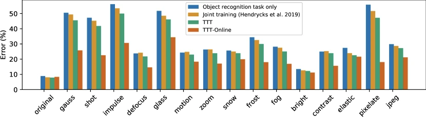
Figure 1 of Sun et al. 2020 (arXiv:1909.13231), reproduced for editorial coverage.

Cluster classification: Inference method · Training method · Theoretical (Sun et al. Theorem 1) · LLM-based (Akyürek et al.) · Representation learning · Benchmark (ARC).

Why these two together. The reviewed user-provided cluster originally listed three papers; on retrieval, two of them (Sun et al. arXiv:1909.13231 and the Hardt-Sun PMLR 2020 entry) reconciled to the same ICML 2020 paper. This article therefore covers the canonical TTT paper (Sun et al. 2020) plus the language-model adaptation (Akyürek et al. 2024). Together they trace one idea across two regimes: TTT as a vision/robustness technique, then TTT as a reasoning/few-shot technique. Reading them side by side surfaces what’s new in the LM era versus what was already present in the 2020 formulation. ^{1 4}

Primary research question (cluster-level). Can a model’s parameters be productively updated on a single unlabeled test input (or a few-shot demonstration set) using a self-supervised or in-context objective, so that the model becomes a better classifier / reasoner for that input than its fixed parameters would suggest?

Core technical claim (cluster-level). Yes, when the auxiliary loss correlates in gradient direction with the main task loss, and when the model has enough capacity (or LoRA adapter capacity) to specialise. Sun et al. 2020 prove a one-step convex-case version of this claim and show empirical correlation $r = 0.93$ between gradient inner product and main-task improvement on CIFAR-10-C. ¹ Akyürek et al. demonstrate the LM analogue: in-context demonstrations of an ARC task, expanded via leave-one-out and invertible geometric augmentations, give the gradient direction needed to specialise a LoRA adapter for that single task. ⁴

Core technical domains and depth. Self-supervised learning (moderate). Multi-task learning (moderate). Convex optimisation theory (moderate). Parameter-efficient fine-tuning, specifically LoRA (deep, in Akyürek et al. coverage). ARC benchmark structure (moderate). Robustness-to-distribution-shift evaluation (deep).

Reader prerequisites. High-school algebra. Familiarity with the idea that a neural network has weights, computes a prediction, and adjusts weights through gradient descent. The Glossary in Section 2.5 covers every other term used in the article (self-supervised, LoRA, gradient correlation, ARC, in-context learning, rotation prediction, distribution shift, leave-one-out, hierarchical voting).

Section 2: TL;DR and executive overview

TL;DR. When a trained machine-learning model meets a hard test input, a corrupted image, a novel reasoning puzzle, it normally just guesses with frozen weights. Test-time training instead lets the model briefly retrain itself on that one input, using a “side task” that doesn’t need a correct answer to learn from (rotating an image and predicting the rotation, or learning from a few example demonstrations). Sun et al. 2020 introduced this for image classification under corruption; Akyürek et al. 2024 showed the same trick works on language-model reasoning, taking a fine-tuned 8B model from $36\%$ to $47\%$ on the ARC reasoning benchmark, and to $61.9\%$ when combined with program-synthesis tools, comparable to average human performance ($60.2\%$). ⁴

Executive summary. Test-time training is a third axis of test-time compute, distinct from chain-of-thought (more tokens) and reinforcement fine-tuning (training-time adjustment to elicit reasoning at inference). TTT spends compute by updating weights on each test input, then making the prediction with those updated weights. The 2020 vision paper proved that the auxiliary loss gradient must correlate with the main loss gradient for this to help, and demonstrated improvements of up to 38% on heavily-corrupted CIFAR-10-C. The 2024 ARC paper transplanted the idea to language models, replacing rotation prediction with in-context-demonstration loss and adding aggressive geometric augmentations. The combined picture: TTT is one of the few techniques that lets a fixed model substantively improve on individual hard inputs without retraining the whole network. ^{1 4}

Five practitioner-relevant takeaways.

• TTT requires a self-supervised auxiliary task whose gradient correlates with the main task. Rotation prediction works for vision; in-context-demonstration loss works for few-shot reasoning. Picking the wrong auxiliary task can degrade main-task performance.
• The Sun et al. Y-shaped architecture (shared feature extractor, two heads) is a structural commitment at training time; you cannot retrofit TTT onto an arbitrary pretrained model without either re-training with an auxiliary head or, in the LM case, using an in-context-demonstration loss that needs no architectural change. ¹
• Akyürek et al. report $\sim$12 hours on an NVIDIA A100 to TTT-process 100 ARC tasks at LoRA rank 128. TTT is expensive at inference; this is its main weakness as a deployment technique. ⁴
• LoRA-per-task is the practical interface for LM TTT: each test instance gets its own freshly-initialised LoRA adapter, trained for 2 epochs against the leave-one-out demonstrations. The base model stays frozen. ⁴
• Hierarchical voting across invertible augmentations (rotations, flips, transpose, color permutations) is what closes the gap to oracle accuracy. Single-augmentation TTT improves modestly; aggregated TTT approaches oracle performance. ⁴

Pipeline overview in text. Sun et al. train a Y-shaped network jointly on the main supervised task (image classification) and the self-supervised rotation-prediction task; at inference, they make 10 gradient steps on the rotation loss for the current test image, updating only the shared feature extractor, then make the classification prediction with the updated extractor. Akyürek et al. start with a fine-tuned LM; at inference, for each ARC task they construct a synthetic training set from the task’s few demonstrations (leave-one-out + invertible augmentations), train a fresh LoRA adapter on that synthetic set for 2 epochs, then predict with the LoRA-adapted model under multiple test-time augmentations and aggregate via hierarchical voting.

Section 2.5: Glossary

Term	Plain-English explanation	First appears in
Test-time training (TTT)	Briefly updating a model’s weights on the test input itself (using a self-supervised loss that doesn’t need a label) before producing the prediction.	Section 1
Self-supervised loss	A training signal that doesn’t require human-labelled answers — the input itself supplies the supervision (e.g., predict the rotation of a rotated image).	Section 1
Distribution shift	The test data comes from a different distribution than the training data (e.g., trained on clean CIFAR-10, tested on corrupted CIFAR-10-C).	Section 1
Rotation prediction	A self-supervised task: rotate an image by 0, 90, 180, or 270 degrees and train the model to predict the rotation as a 4-way classification.	Section 1
ARC benchmark	The Abstraction and Reasoning Corpus, a benchmark of grid-puzzle tasks where each task has a few input-output examples and the model must infer the transformation rule.	Section 1
LoRA	Low-Rank Adaptation: a parameter-efficient fine-tuning method that adds small trainable matrices to a frozen pretrained model.	Section 1
In-context demonstrations	A few example input-output pairs shown to a language model at inference, from which it should infer the task.	Section 1
Leave-one-out	A data-construction trick: given $K$ examples, build $K$ synthetic tasks where each example becomes the held-out test case and the other $K-1$ become demonstrations.	Section 1
Hierarchical voting	A two-stage majority-vote aggregation that first picks the top predictions within each augmentation, then aggregates across augmentations.	Section 2
Gradient correlation	The inner product between two loss-function gradients. Positive correlation means stepping to reduce one loss tends to reduce the other.	Section 6
Y-shaped architecture	A neural network with a shared trunk that branches into two heads, one for each task in multi-task training.	Section 5
Chain-of-thought (CoT)	An LLM prompting style that asks the model to generate intermediate reasoning tokens before the final answer; spends test-time compute on more tokens.	Section 4
Reinforcement fine-tuning (RFT)	A training-time technique that adjusts an LLM with reinforcement learning to make it elicit reasoning at inference; the weights are fixed at deployment.	Section 4
[Analysis] label	The publication’s own reasoned assessment, distinct from what the paper itself claims.	Throughout
[Reviewer Perspective] label	A critical or speculative assessment that goes beyond what the paper proves, often grounded in independent commentary.	Sections 11, 12

The remaining claim-taxonomy markers, [Reconstructed], [External comparison], and the “From the paper:” prefix, follow the conventions in Section 0 of the publication’s paper-review pillar style guide. “From the paper” content is directly supported by the cited paper’s text, equations, tables, or figures; [Reconstructed] content is faithfully reconstructed from partial paper disclosure; [External comparison] content compares to named prior work or general knowledge outside either paper.

Section 3: Problem formalisation

Notation table.

Symbol	Type	Meaning	First appears in
$x$	input	Test input (image for Sun et al.; ARC task demonstrations + test grid for Akyürek et al.)	Section 3
$y$	label	Main-task target (class label; output grid)	Section 3
$\theta_e$	parameters	Shared feature-extractor weights	Section 5
$\theta_m$	parameters	Main-task head weights (classifier)	Section 5
$\theta_s$	parameters	Self-supervised head weights (rotation classifier)	Section 5
$\ell_m$	loss	Main supervised loss (cross-entropy)	Section 5
$\ell_s$	loss	Self-supervised loss (rotation prediction or LM next-token on demos)	Section 5
$\eta$	scalar	Inner learning rate at test time	Section 6
$K$	integer	Number of demonstration examples per ARC task	Section 5
$r$	integer	LoRA rank	Section 5
$\alpha$	integer	LoRA scaling parameter	Section 5
$\mathcal{T}$	set	Set of invertible geometric transformations	Section 5
$\beta, G$	scalars	Loss smoothness constant and gradient norm bound (Theorem 1)	Section 6

Formal problem statement (Sun et al.). Given a training distribution $\mathcal{D}_{\text{train}}$ and a (potentially different) test distribution $\mathcal{D}_{\text{test}}$, train a predictor that achieves low expected main-task loss on $\mathcal{D}_{\text{test}}$. The key constraint: only individual unlabeled test samples are observed at test time; no batch of target-distribution data is available, and no labels are revealed. ¹ The objective is to minimise $\mathbb{E}_{(x,y)\sim\mathcal{D}_{\text{test}}}[\ell_m(x,y;\theta(x))]$ where the decision rule’s parameters $\theta(x)$ are allowed to depend on the test input, a sample-dependent parameter setting rather than the standard fixed $\theta$.

Formal problem statement (Akyürek et al.). Given a base LM fine-tuned on ARC-like tasks, and a test ARC task consisting of $K$ input-output demonstration pairs $(x_1, y_1), \ldots, (x_K, y_K)$ plus a held-out test input $x_{\text{test}}$, produce $y_{\text{test}}$. The constraint: the test task has a structurally novel transformation rule not seen during fine-tuning; the model must therefore infer the rule from $K$ examples and apply it. ARC explicitly disallows pretraining on the test task; the demonstrations are the only supervision available for that task. ¹⁰

Explicit assumptions.

• (Sun et al.) The self-supervised auxiliary task is structurally relevant to the main task. The paper’s Theorem 1 makes this concrete: positive gradient correlation between $\ell_m$ and $\ell_s$ at the current parameter. Without this correlation, TTT can hurt rather than help. [Analysis] Potentially strong assumption, verifying gradient correlation across an entire test distribution at design time requires either theoretical justification (the auxiliary task and main task share features) or empirical measurement on a held-out validation set. ¹
• (Sun et al.) The shift in $\mathcal{D}_{\text{test}}$ does not destroy the self-supervised signal. Rotation prediction works on corrupted images because rotation is still well-defined despite gaussian noise or pixelation; it would fail if the corruption itself involved rotation. [Analysis] Realistic for the corruption benchmarks tested; would not generalise to all conceivable shifts.
• (Akyürek et al.) The base model has been fine-tuned on ARC-format tasks with a curriculum that includes leave-one-out training and invertible-transformation augmentations. TTT-from-scratch on a generic instruction-tuned LM is shown in their ablations to be substantially weaker. ⁴
• (Akyürek et al.) Test-time augmentation is invertible, so predictions on transformed inputs can be back-transformed to a canonical space for aggregation. Non-invertible augmentations (e.g., cropping) would break the voting scheme. ⁴

Formal complexity arguments. Sun et al. perform 10 inner gradient steps on a ResNet-26 per test sample; this multiplies inference cost by roughly $10\times$ relative to standard forward-only inference ([Analysis], the paper does not report wall-clock cost explicitly, but the gradient-step count is reported in Section 4.1). ¹ Akyürek et al. report $\sim 12$ hours on an A100 for 100 ARC tasks with full TTT and augmentation aggregation; the per-task cost is therefore approximately 7 minutes of A100 time, which the authors explicitly note disqualifies them from the official ARC leaderboard’s compute budget. ⁴

Section 4: Motivation and gap

Real-world problem with a concrete example. Image classifiers trained on clean ImageNet routinely lose 30-50 percentage points of accuracy when tested on the same images with realistic corruptions (motion blur, gaussian noise, jpeg compression). The deployment reality is that test images frequently come from this corrupted distribution, phone cameras at night, security cameras at dusk, medical scanners with calibration drift. Standard solutions either retrain on every conceivable corruption (combinatorially expensive) or apply domain adaptation with target-domain data (which assumes target-domain labels or at least a batch of target-domain samples). ¹²

Existing approaches and their failure modes (per Sun et al.’s related work).

• Domain adaptation: needs a batch of target-domain examples and explicit knowledge of the shift. Fails when each test input is potentially from a different distribution.
• Robust training / data augmentation: helps on covered corruptions but does not generalise to unseen shifts. Sun et al. demonstrate this empirically, their joint-training baseline already incorporates auxiliary-task augmentation, and TTT still improves on top of it. ¹
• Self-supervised pretraining: produces fixed features at deployment; cannot adapt to a specific test sample.

For language-model reasoning, the analogous gap (per Akyürek et al.’s framing): chain-of-thought and majority-vote at inference both spend compute generating more tokens with fixed weights. They cannot recover information that the fine-tuned weights lack about a specific novel transformation rule. RFT pushes the model toward more reasoning behaviour at training time, but again deploys with fixed weights. None of these techniques update the weights on the specific test puzzle. ^{4 15 16}

Gap the papers claim to fill. Sun et al.: a general test-time adaptation mechanism that works on a single unlabeled sample, requires no target-domain batch, and does not assume knowledge of the shift type. Akyürek et al.: a test-time adaptation mechanism for language models that lifts performance on structurally novel reasoning tasks by a factor far larger than is achievable through prompting-only test-time compute.

Practical stakes. A deployable robustness technique that operates per-sample is qualitatively different from a deployable robustness technique that requires a target-domain batch. The latter is unusable when the test distribution is unknown or per-sample-varying. For LM reasoning, a technique that gains $\sim 30$ percentage points on ARC is large enough to change which model class is competitive on benchmarks the standard prompting toolkit has saturated near low accuracy. ⁴

[External comparison] Position in the broader research landscape. TTT sits alongside three other test-time compute approaches: chain-of-thought (Wei et al. 2022, more tokens, fixed weights), self-consistency / majority-vote sampling (Wang et al. 2022, multiple decodes, fixed weights), and verifier-guided search (Snell et al. 2024, beam-search style aggregation with a process reward model). ^{15 16} TTT is the only one of the four that updates weights at inference. It is also the only one with a published theoretical guarantee (Sun et al. Theorem 1) of when it provably helps. The fully-online Tent paper (Wang et al. 2021) updates batch-norm statistics at test time by entropy minimisation, which is a special case of the TTT pattern with a different self-supervised signal. ⁸

Section 5: Method overview

Sun et al. 2020: Y-shaped architecture with rotation auxiliary

Plain-English intuition: imagine a network with one body and two heads. The body extracts features; one head predicts the class, the other head predicts the rotation. During training, the body learns features that serve both heads. At test time, the rotation head and the body collaborate to learn from the rotation of the single test image, updating the body. Then the (now slightly retrained) body feeds the classifier head, which makes the prediction.

Component 1: Y-shaped network. [New for this paper, building on Gidaris et al. 2018’s rotation pretext task.] ¹⁴ The architecture splits a ResNet into a shared trunk parametrised by $\theta_e$ and two heads: $\theta_m$ for the main classification task and $\theta_s$ for the rotation-prediction task. The branch point is a hyperparameter; the paper uses a ResNet-26 with the branch after the first ResBlock group.

Component 2: Joint training objective. During training, all parameters are updated by minimising the joint loss $\min_{\theta_e, \theta_m, \theta_s} \frac{1}{n} \sum_{i=1}^{n} \left[ \ell_m(x_i, y_i; \theta_m, \theta_e) + \ell_s(x_i; \theta_s, \theta_e) \right]$ where $\ell_s$ is the four-way cross-entropy on the rotation-prediction task. The rotation labels are produced automatically by rotating each training image to one of four canonical orientations.

Component 3: Standard TTT update. At inference, given a single test image $x$, the procedure freezes $\theta_m$ and $\theta_s$ and updates only $\theta_e$ by gradient descent on the self-supervised loss: $\theta_e' = \theta_e - \eta \nabla_{\theta_e} \ell_s(x; \theta_s, \theta_e)$ applied for 10 steps with $\eta = 0.001$. The main prediction is then made with the updated $\theta_e'$. ¹

Component 4: Online TTT variant. When test images arrive as a stream, the parameters from the previous test sample initialise the inner-loop optimisation for the next sample, accumulating adaptation. Sun et al. report this yields larger improvements (>24% on noise, 38% on pixelation) than restarting from $\theta_e$ each sample. ¹

Design rationale. Rotation prediction was chosen because Gidaris et al. 2018 had already shown it learns semantically meaningful features for classification. The Sun et al. contribution is recognising that any such auxiliary task can be used adaptively at test time rather than only at pretraining. ¹⁴ What breaks if removed: without the auxiliary head, there is no gradient signal for $\theta_e$ at test time (the main loss is unavailable because labels are unknown).

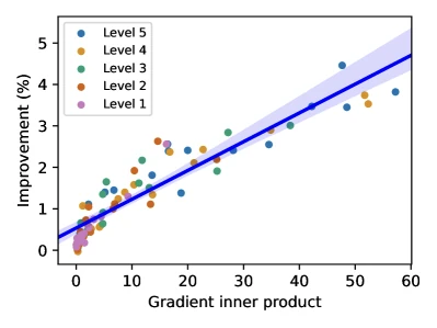
Figure 4 of Sun et al. 2020 (arXiv:1909.13231), reproduced for editorial coverage. The scatter is the empirical validation of Theorem 1’s gradient-correlation condition.

Akyürek et al. 2024: Per-task LoRA TTT for ARC

Plain-English intuition: for each ARC puzzle, the model gets a few example input-output grids. The Akyürek et al. recipe: take those examples, multiply them by aggressive augmentations (rotate the grids, flip them, recolor them, leave each example out in turn) to get a much larger synthetic training set; train a fresh tiny adapter on that synthetic set; predict with the adapter on the test grid, again under multiple augmentations; aggregate the predictions by majority vote.

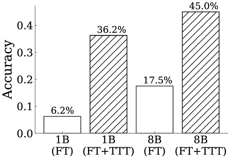
Figure 1 of Akyürek et al. 2024 (arXiv:2411.07279), reproduced for editorial coverage. Left: accuracy improvements across model sizes. Right: a representative task the fine-tuned LM solves only after TTT.

Component 1: Leave-one-out task augmentation. [New for ARC; the leave-one-out idea is general but applied here in a specific construction.] ⁴ For a task with $K$ demonstrations, build $K$ synthetic tasks by removing each demonstration in turn and using it as the test case. Add two random permutations of each leave-one-out task. This multiplies the effective TTT training set by approximately $3K$.

Component 2: Invertible geometric augmentation. Apply rotations ($90°, 180°, 270°$), horizontal and vertical flips, transpose, reflections with prepend or append, random translations up to 4 cells, resolution scaling, and color permutations. Each augmentation is invertible so test predictions can be back-transformed for voting.

Component 3: Per-task LoRA training. [Adopted from Hu et al. 2021 LoRA, adapted for per-instance test-time use.] ¹⁷ Each test instance gets a freshly-initialised LoRA adapter of rank 128 with $\alpha = 16$, targeting query/value projections, MLP layers, and output projections. The adapter trains via AdamW for 2 epochs at batch size 2, learning rate $5 \times 10^{-5}$ to $1 \times 10^{-4}$. The base LM stays frozen.

Component 4: Training loss. The objective sums next-token language-model loss over the demonstrations (predicting each $y_n$ from the prior $n-1$ demonstrations starting from $n=2$) plus the prediction loss on the held-out test demonstration: $\sum_{d \in \mathcal{D}_{\text{TTT}}} \left[ \sum_{n=2}^{K} \mathcal{L}_{\text{LM}}(y_n \mid x_1, y_1, \ldots, x_n) + \mathcal{L}_{\text{LM}}(y_{\text{test}} \mid x_1, y_1, \ldots, x_K, x_{\text{test}}) \right]$ This shape forces the adapter to model the transformation rule rather than memorise a single example. ⁴

Component 5: Hierarchical voting at inference. For the actual test query, the model runs under each invertible augmentation, producing one prediction per augmentation. The voting proceeds in two stages: (i) intra-transformation voting, picking the top-3 predictions within each transformation group, supplemented with row-based and column-based majority voting if fewer than 3 unique predictions exist; (ii) global voting, aggregating transformation-specific candidates to select the top-2 most frequent predictions, with the identity transformation prioritised in ties. ⁴

Design rationale. ARC tasks are by construction structurally novel; the base LM has not seen the specific transformation rule. The few demonstrations carry the rule. The leave-one-out + augmentation procedure converts those few demonstrations into enough training signal to let a small adapter specialise. What breaks if removed: the ablation in Figure 3 of the paper shows that removing in-context format degrades TTT dramatically, and removing geometric augmentations halves the improvement. ⁴

Figure 2 of Akyürek et al. 2024 (arXiv:2411.07279), reproduced for editorial coverage. The pipeline transforms K demonstrations into 3K x augmentation_count training signal for the per-task LoRA.

Section 6: Mathematical contributions

MATH ENTRY 1: Sun et al. joint training objective.

• Source: Section 3.1, equation 1 of Sun et al. 2020.
• What it is: the loss used during training, summing the main classification loss and the self-supervised rotation loss across the dataset.
• Formal definition: $\min_{\theta_e, \theta_m, \theta_s} \frac{1}{n} \sum_{i=1}^{n} \left[ \ell_m(x_i, y_i; \theta_m, \theta_e) + \ell_s(x_i; \theta_s, \theta_e) \right]$
• Each term explained, with dimensional analysis:
  • $x_i$ is an image, a tensor of shape $[3, H, W]$ (RGB).
  • $y_i$ is a scalar class label in $\\{1, \ldots, C\\}$.
  • $\theta_e$ are the shared trunk weights, in $\mathbb{R}^{\mid \theta_e\mid }$ where $\mid \theta_e\mid$ is in the millions for a ResNet-26.
  • $\ell_m$ outputs a scalar; $\ell_s$ outputs a scalar; their sum is a scalar; the average over $n$ is a scalar.
  • The implicit weighting between $\ell_m$ and $\ell_s$ is 1:1; Sun et al. do not introduce a Lagrange multiplier.
• Worked numerical example: take a mini-batch of $n=2$ images, $C=10$ classes, 4 rotations. Suppose $\ell_m$ on image 1 is 0.6, on image 2 is 0.4. Suppose $\ell_s$ (rotation cross-entropy) is 1.2 on image 1, 1.0 on image 2. The joint loss is $\frac{1}{2}[(0.6 + 1.2) + (0.4 + 1.0)] = \frac{1}{2}(1.8 + 1.4) = 1.6$. Gradient descent updates $\theta_e$ to reduce this scalar.
• Role: shapes the feature trunk to be jointly useful for classification and rotation prediction. The two-task pressure during training is what makes the test-time adaptation work, the trunk has learned to encode features that both heads benefit from.
• Edge cases: if $\ell_s$ overwhelmingly dominates (because rotation is much easier than classification at initialisation), the joint training collapses to rotation prediction. Sun et al. note this empirically does not happen for the auxiliary losses they tried.
• Novelty: [Adapted], joint multi-task training is standard; the specific use of rotation as the auxiliary task is adopted from Gidaris et al. 2018. ¹⁴
• Why it matters: the test-time update relies on the trunk having useful rotation-prediction gradients at any point in parameter space, which is only true if the trunk was trained to support rotation prediction jointly.

MATH ENTRY 2: Sun et al. test-time update.

• Source: Section 3.2, equation 3 of Sun et al. 2020.
• What it is: at inference, take a single test image, compute its rotation loss, and step the trunk weights to reduce that loss.
• Formal definition: $\theta_e^{(t+1)} = \theta_e^{(t)} - \eta \nabla_{\theta_e} \ell_s(x; \theta_s, \theta_e^{(t)})$ applied for $T = 10$ steps with $\eta = 0.001$.
• Each term explained, with dimensional analysis:
  • $x$ is the test image, a tensor in $\mathbb{R}^{3 \times H \times W}$. To compute $\ell_s$, the procedure forms four copies $x^{(0°)}, x^{(90°)}, x^{(180°)}, x^{(270°)}$ and runs the rotation head on each.
  • $\nabla_{\theta_e} \ell_s$ has the same shape as $\theta_e$, millions of partial derivatives.
  • $\eta$ is a scalar; the product $\eta \nabla \ell_s$ is a parameter update vector of the same shape as $\theta_e$.
• Worked numerical example: take a toy trunk with $\mid \theta_e\mid = 4$ parameters, $\theta_e^{(0)} = [0.5, -0.2, 0.1, 0.3]$. Suppose the rotation loss gradient at a single test image is $\nabla_{\theta_e} \ell_s = [0.1, -0.05, 0.2, 0.0]$ and $\eta = 0.001$. After one step: $\theta_e^{(1)} = [0.5 - 0.0001, -0.2 + 0.00005, 0.1 - 0.0002, 0.3] = [0.4999, -0.19995, 0.0998, 0.3]$. After 10 such steps, the trunk has shifted by roughly $0.001 \times 10 \times \\mid \nabla \ell_s\\mid \approx 0.0023$ in parameter norm. The shift is small but consistent in a direction that, by Theorem 1, also reduces $\ell_m$ on this test image.
• Role: produces a sample-dependent parameter setting $\theta_e(x)$ that is better for predicting this particular $x$ than the population-optimal $\theta_e$.
• Edge cases: if the gradient $\nabla_{\theta_e} \ell_s$ is uncorrelated or anti-correlated with $\nabla_{\theta_e} \ell_m$, the update degrades main-task performance. Theorem 1 below formalises the boundary.
• Novelty: [New], the test-time gradient-step idea on a self-supervised auxiliary is the paper’s central contribution.
• Why it matters: this is the specific equation that defines test-time training. Everything else (online variant, masked-autoencoder variant in Gandelsman et al. 2022, LM variant in Akyürek et al. 2024) is a different choice of $\ell_s$ or a different parameter subset to update. ⁶

MATH ENTRY 3: Sun et al. Theorem 1, gradient-correlation guarantee.

• Source: Theorem 1, Section 3.3 of Sun et al. 2020.
• What it is: a sufficient condition for one TTT step to provably reduce the main task loss on the current test sample.
• Formal statement (paraphrased): assume $\ell_m$ and $\ell_s$ are convex, $\beta$-smooth in $\theta$, with gradient norms bounded by $G$. If at parameter $\theta$ the gradient inner product satisfies $\langle \nabla_\theta \ell_m(x, y; \theta), \nabla_\theta \ell_s(x; \theta) \rangle > \varepsilon$ then a gradient step on $\ell_s$ with step size $\eta = \varepsilon / (\beta G^2)$ strictly decreases $\ell_m(x, y; \theta)$.
• Each term explained:
  • $\langle \cdot, \cdot \rangle$ is the Euclidean inner product over the parameter vector. It is positive when the two gradients point in roughly the same direction.
  • $\beta$ is the smoothness constant: $\\mid \nabla \ell(\theta_1) - \nabla \ell(\theta_2)\\mid \leq \beta \\mid \theta_1 - \theta_2\\mid$.
  • $G$ bounds $\\mid \nabla \ell_s\\mid$; combined with $\beta$, it controls how aggressive the step can be before second-order curvature ruins the guarantee.
  • $\varepsilon > 0$ is any positive constant; the theorem says the step size scales inversely with $\varepsilon$, so small correlation requires a small step.
• Proof sketch (every step, no hand-waving):
  • Step 1: by $\beta$-smoothness of $\ell_m$, for any update $\Delta \theta$, $\ell_m(\theta + \Delta\theta) \leq \ell_m(\theta) + \langle \nabla \ell_m(\theta), \Delta\theta \rangle + \frac{\beta}{2} \\mid \Delta\theta\\mid ^2$. This is the standard smoothness upper bound; it is a consequence of integrating the gradient along the line segment from $\theta$ to $\theta + \Delta\theta$ and applying the Lipschitz-gradient property.
  • Step 2: substitute $\Delta\theta = -\eta \nabla \ell_s(\theta)$, the TTT update. The bound becomes $\ell_m(\theta + \Delta\theta) \leq \ell_m(\theta) - \eta \langle \nabla \ell_m, \nabla \ell_s \rangle + \frac{\beta \eta^2}{2} \\mid \nabla \ell_s\\mid ^2$.
  • Step 3: use the hypothesis $\langle \nabla \ell_m, \nabla \ell_s \rangle > \varepsilon$ and the gradient-norm bound $\\mid \nabla \ell_s\\mid \leq G$. The bound becomes $\ell_m(\theta + \Delta\theta) < \ell_m(\theta) - \eta \varepsilon + \frac{\beta \eta^2 G^2}{2}$.
  • Step 4: choose $\eta = \varepsilon / (\beta G^2)$. Substituting, the negative term becomes $-\varepsilon^2 / (\beta G^2)$ and the positive curvature term becomes $\frac{\beta \cdot \varepsilon^2 / (\beta G^2)^2 \cdot G^2}{2} = \varepsilon^2 / (2\beta G^2)$. The net change is $\ell_m(\theta + \Delta\theta) - \ell_m(\theta) < -\varepsilon^2 / (\beta G^2) + \varepsilon^2 / (2\beta G^2) = -\varepsilon^2 / (2\beta G^2)$.
  • Step 5: the right-hand side is strictly negative, so $\ell_m$ strictly decreased after the step. $\blacksquare$
• Worked numerical example: suppose $\varepsilon = 0.1$, $\beta = 10$, $G = 1$. Then $\eta = 0.1 / 10 = 0.01$. The guaranteed decrease is at least $\varepsilon^2 / (2\beta G^2) = 0.01 / 20 = 5 \times 10^{-4}$. The theorem is a worst-case bound; empirical decreases are typically larger.
• Role: justifies the empirical observation that TTT helps. The condition is checkable post-hoc, Sun et al. measure the gradient inner product on a held-out validation set and report Pearson correlation $r = 0.93$ between inner-product magnitude and main-task improvement (Section 4.4). ¹
• Edge cases: the theorem assumes convexity, which deep networks do not satisfy. Sun et al. acknowledge this gap and treat the theorem as a one-step local result valid in a small neighbourhood of $\theta$. The empirical correlation supports the local-convex intuition extending to deep networks in practice.
• Novelty: [New], this is the paper’s theoretical contribution.
• Why it matters: it converts TTT from an empirical trick into a principled procedure with a checkable correctness condition.

MATH ENTRY 4: Akyürek et al. TTT loss.

• Source: Section 3.2 of Akyürek et al. 2024.
• What it is: the loss used to train the per-task LoRA adapter during TTT.
• Formal definition: $\mathcal{L}_{\text{TTT}}(\phi) = \sum_{d \in \mathcal{D}_{\text{TTT}}} \left[ \sum_{n=2}^{K} \mathcal{L}_{\text{LM}}(y_n \mid x_1, y_1, \ldots, x_n; \theta_{\text{base}}, \phi) + \mathcal{L}_{\text{LM}}(y_{\text{test}} \mid x_1, y_1, \ldots, x_K, x_{\text{test}}; \theta_{\text{base}}, \phi) \right]$
• Each term explained, with dimensional analysis:
  • $\phi$ are the LoRA adapter weights, in $\mathbb{R}^{r \times d} \times \mathbb{R}^{d \times r}$ pairs across targeted modules; with $r=128$ and an 8B model, $\mid \phi\mid$ is on the order of $10^7$.
  • $\theta_{\text{base}}$ are the frozen base-model weights, on the order of $8 \times 10^9$ for the 8B model.
  • $\mathcal{D}_{\text{TTT}}$ is the synthetic dataset of leave-one-out tasks, of size approximately $3K \times \mid \mathcal{T}\mid$ where $\mid \mathcal{T}\mid$ is the augmentation count.
  • $\mathcal{L}_{\text{LM}}$ is the standard next-token cross-entropy summed over output tokens.
• Worked numerical example: suppose $K = 4$ demonstrations and $\mid \mathcal{T}\mid = 8$ augmentations (rotations + flips). $\mid \mathcal{D}_{\text{TTT}}\mid \approx 3 \times 4 \times 8 = 96$ synthetic tasks. For each task, the inner sum runs $n = 2, 3, 4$ (three demonstration-prediction losses), plus the test-prediction loss, four LM losses per task. Total loss-term count per epoch is $96 \times 4 = 384$. At batch size 2 and 2 epochs, that’s $384$ training steps per test instance.
• Role: provides the gradient signal to specialise $\phi$ to this specific test task.
• Edge cases: when $K = 1$ (only one demonstration), the leave-one-out construction collapses and the inner sum is empty; only the test-prediction term survives. Akyürek et al. report ARC tasks always have $K \geq 2$. ⁴
• Novelty: [New] for the leave-one-out + invertible-augmentation construction; [Adopted] for the LoRA training objective itself.
• Why it matters: this loss is what converts a handful of demonstrations into enough training signal for a rank-128 adapter to learn the task-specific transformation.

Section 7: Algorithmic contributions

ALGORITHM ENTRY 1: Sun et al. Standard TTT (the headline algorithm).

• Source: Algorithm 1 of Sun et al. 2020.
• Purpose: adapt the trunk weights to a single test sample using rotation prediction, then make the main-task prediction.
• Inputs:
  • Test image $x \in \mathbb{R}^{3 \times H \times W}$.
  • Trained parameters $\theta_e, \theta_m, \theta_s$.
  • Inner steps $T = 10$, inner learning rate $\eta = 0.001$.
• Outputs:
  • Main-task prediction $\hat{y}$.
• Pseudocode:

  function StandardTTT(x, theta_e, theta_m, theta_s, T=10, eta=0.001):
      theta_e' = theta_e                                     # initialise from training params
      for t in 1..T:                                         # T inner steps
          x_0, x_90, x_180, x_270 = rotate_all_four(x)       # construct rotation batch
          features = trunk(x_0|x_90|x_180|x_270; theta_e')   # forward through trunk
          rot_logits = rotation_head(features; theta_s)      # rotation prediction
          rot_labels = [0, 1, 2, 3]                          # ground truth from rotations
          ell_s = cross_entropy(rot_logits, rot_labels)
          grad = backprop(ell_s, w.r.t. theta_e')
          theta_e' = theta_e' - eta * grad                   # gradient step on trunk
      features_main = trunk(x; theta_e')                     # forward with updated trunk
      logits = main_head(features_main; theta_m)             # main prediction
      return argmax(logits)

• Hand-traced example on minimal input. Take a 3-class toy problem, a trunk with 4 parameters $\theta_e = [0.5, -0.2, 0.1, 0.3]$. Test image $x$. Step 1 of the inner loop: $x_0, x_{90}, x_{180}, x_{270}$ are computed. The rotation head with the current trunk outputs logits $[0.1, 0.2, 0.0, 0.3], [0.3, 0.1, 0.0, 0.2], [0.2, 0.3, 0.1, 0.0], [0.1, 0.0, 0.4, 0.1]$, i.e., it currently predicts the rotation poorly. The cross-entropy loss is computed against labels $[0, 1, 2, 3]$ and back-propagated; suppose the gradient is $[0.1, -0.05, 0.2, 0.0]$. Update: $\theta_e' = [0.4999, -0.19995, 0.0998, 0.3]$ after step 1. After 10 such steps, $\theta_e'$ has shifted by approximately $\eta T \\mid \nabla\\mid \approx 0.001 \times 10 \times 0.23 = 0.0023$ in parameter-norm units. The main head then runs with $\theta_e'$ and outputs class logits $[1.2, 0.8, 0.9]$; the prediction is class 0.
• Complexity: $T \cdot$ (forward + backward) per test sample, with the forward batched over 4 rotations. Roughly $10\times$ the single-image inference cost. Memory: needs to retain activations for back-propagation, also $\sim 10\times$ standard inference.
• Hyperparameters: $T = 10$ inner steps, $\eta = 0.001$ inner LR (Section 4.1 of paper). Sensitivity: the paper reports stable behaviour over $T \in [5, 20]$ and $\eta \in [5 \times 10^{-4}, 5 \times 10^{-3}]$. Larger $T$ risks over-fitting to the rotation task.
• Failure modes: if $\nabla \ell_s$ and $\nabla \ell_m$ are anti-correlated at $\theta_e$ for this $x$, the update hurts the main task. Empirically rare for the rotation task on natural images but real for adversarial corruptions designed to flip the gradient direction.
• Novelty: [New], this is the paper’s headline algorithm.
• Transferability: [Analysis] The algorithm generalises to any (main task, auxiliary task) pair where joint training makes the trunk useful for both and gradients correlate. The masked-autoencoder variant (Gandelsman et al. 2022) replaces rotation with MAE reconstruction and the RNN-with-expressive-hidden-state variant (Sun et al. 2024) treats the hidden state as a per-token TTT optimiser. ^{6 7}

ALGORITHM ENTRY 2: Akyürek et al. ARC-TTT inference pipeline.

• Source: Section 3 of Akyürek et al. 2024.
• Purpose: for each ARC task, train a per-task LoRA, then aggregate predictions across augmentations via hierarchical voting.
• Inputs:
  • Demonstrations $\\{(x_k, y_k)\\}_{k=1}^{K}$, test input $x_{\text{test}}$.
  • Fine-tuned base LM $\theta_{\text{base}}$, augmentation set $\mathcal{T}$.
  • LoRA rank $r = 128$, $\alpha = 16$, AdamW, learning rate $5 \times 10^{-5}$, 2 epochs, batch size 2.
• Outputs:
  • Predicted test output $\hat{y}_{\text{test}}$.
• Pseudocode:

  function ARC_TTT(demos, x_test, theta_base, T_set, r=128, alpha=16):
      # Step 1: build synthetic TTT training set
      D_TTT = []
      for j in 1..K:                                          # leave-one-out
          D_TTT.append(demos[1..j-1] + demos[j+1..K], demos[j].x, demos[j].y)
      D_TTT += permute_demos(D_TTT, 2 random perms each)      # 3x expansion
      D_TTT_aug = [apply_transform(t, d) for d in D_TTT, t in T_set]   # |T_set|x
  
      # Step 2: train per-task LoRA
      phi = LoRA_init(r, alpha)                               # fresh adapter
      phi = AdamW_train(phi, theta_base, D_TTT_aug,
                        lr=5e-5, epochs=2, batch=2)
  
      # Step 3: augmented inference
      predictions_by_transform = {}
      for t in T_set:
          x_test_t = apply_transform(t, x_test)
          y_hat_t  = LM_generate(theta_base + phi, demos_t, x_test_t)
          y_hat    = inverse_transform(t, y_hat_t)
          predictions_by_transform[t] = y_hat
  
      # Step 4: hierarchical voting
      intra = {}
      for t in T_set:
          intra[t] = top3_with_row_col_fallback(predictions_by_transform[t])
      candidates = flatten([intra[t] for t in T_set])
      return top2_majority(candidates, tiebreak=identity)

• Hand-traced example on minimal input. Suppose $K = 3$ demos. Leave-one-out yields 3 tasks; two random permutations yields 9 synthetic tasks. Augmentation set $\mathcal{T} = \\{I, R_{90}, R_{180}, R_{270}, F_h, F_v, T, P\\}$ (identity, three rotations, two flips, transpose, color permutation) gives $\mid T\mid = 8$. $D_{\text{TTT}} = 9 \times 8 = 72$ training tasks. Each task has 2 demo-prediction losses plus 1 test-prediction loss = 3 losses, so $72 \times 3 = 216$ loss terms per epoch. 2 epochs = 432 gradient steps at batch size 2 ($\approx 216$ optimiser steps). At inference, 8 augmented test predictions are produced; hierarchical voting picks top-3 within each (24 candidates), then global top-2.
• Complexity: dominated by the LoRA training inner loop. Akyürek et al. report $\sim 12$ hours on a single A100 for 100 ARC tasks, i.e. $\sim 7$ minutes per task. Inference (8 generations + voting) is a small fraction.
• Hyperparameters: rank 128, $\alpha = 16$, AdamW, LR in $[5 \times 10^{-5}, 10^{-4}]$, 2 epochs, batch 2. Sensitivity: ablations in Figure 3 show rank below 64 degrades, learning rate above $5 \times 10^{-4}$ overshoots, more than 3 epochs over-fits. ⁴
• Failure modes: when the demonstrations are ambiguous (multiple consistent transformation rules), augmented voting can lock in a wrong rule. The authors report this is the dominant residual error mode in their qualitative analysis.
• Novelty: [New], specific combination of leave-one-out + invertible augmentation + per-task LoRA + hierarchical voting is the paper’s algorithmic contribution.
• Transferability: [Analysis] The per-task-LoRA pattern generalises to any few-shot setting where (a) demonstrations contain enough signal for an adapter to specialise and (b) invertible augmentations exist. It is less obvious that the approach transfers to natural-language reasoning where augmentations are non-trivial to define invertibly.

Section 8: Specialised design contributions

Subsection 8A: LLM / prompt design

For Akyürek et al., the LM input is the standard few-shot ARC format: a sequence of input-output grid pairs followed by a test input grid. The model is trained to produce the test output grid token-by-token. The “prompt” is implicit in the demonstration tokens; there is no separate natural-language instruction.

PROMPT ENTRY 1: ARC few-shot demonstration sequence (Akyürek et al.)
- Source: Akyürek et al. 2024, Section 3.2, Figure 4
- Role: input format for both TTT training and inference
- Prompt type: Few-shot (in-context demonstrations only, no natural-language preamble)
- Components in order: [demo_1.x][SEP][demo_1.y][DEMO_SEP] ... [demo_K.x][SEP][demo_K.y][DEMO_SEP][test.x][SEP]
- Input schema: ARC grid tokens (color indices 0-9, separated by row markers)
- Output schema: same grid-token format for the predicted output
- Reconstructed template (the paper does not publish the exact tokenisation):
  [Reconstructed] "Example 1 input: {x_1} output: {y_1}\nExample 2 input: {x_2} output: {y_2}\n... \nTest input: {x_test} output:"
- Failure handling: if the model outputs malformed grid tokens, the paper reports the prediction is voted out at the hierarchical-voting stage.
- Design rationale: forces the LM to model transformation rules as autoregressive sequence prediction over grids.
- Complexity: prompt length grows linearly with K demonstrations and grid size.
- Novelty: [Adopted], the in-context demonstration format follows the ARC-format conventions used by BARC (Li et al. 2024) and prior LM-on-ARC work.<FootnoteRef n={11} />
- Transferability: [Analysis] The exact format choice is benchmark-specific; the principle (use the few-shot demo loss as the TTT signal) generalises.

Sun et al. is a vision paper, so PROMPT ENTRY does not apply to it.

Subsection 8B: Architecture-specific details

Sun et al.: ResNet-26 with group-normalisation, branch after the first ResBlock group. The rotation head is a small classifier (single linear layer after global average pooling). The main head is the standard classification linear layer. ¹

Akyürek et al.: LoRA targets the query and value projections within self-attention, the gate/up/down MLP projections, and the output (lm_head) projection. Other layers (embeddings, layernorm) are frozen. The base model is the 1B and 8B sizes of an open-weights LM family (the paper uses Llama-family fine-tuned variants). ⁴

Subsection 8C: Training specifics

Sun et al. training: standard ResNet-26 schedule on CIFAR-10 (SGD, weight decay $5 \times 10^{-4}$, learning rate 0.1 with cosine annealing). Auxiliary rotation labels generated on-the-fly. Training cost is essentially the same as a single-task ResNet because the rotation head is cheap.

Akyürek et al. training: a base fine-tuning stage on ARC-like tasks (ReARC + LLM-generated synthetic tasks + BARC’s training mixture) precedes TTT. The base fine-tune uses standard supervised LM training; details in their Appendix B. The per-instance TTT uses the hyperparameters listed in Algorithm Entry 2 above.

Subsection 8D: Inference / deployment specifics

Sun et al. inference: 10 gradient steps per test image, $\sim 10\times$ inference cost. The online variant carries state forward across the test stream, which the authors note matches real deployment for streaming scenarios (security cameras, autonomous-vehicle perception).

Akyürek et al. inference: $\sim 7$ minutes per ARC task on an A100, dominated by the LoRA training inner loop. The authors explicitly acknowledge this disqualifies them from the official ARC leaderboard’s compute budget, which limits per-task inference to a small number of seconds. ⁴

Section 9: Experiments and results

Datasets

• CIFAR-10-C (Sun et al.): 15 corruption types at 5 severity levels, applied to CIFAR-10 test images. Standard robustness benchmark. ¹²
• ImageNet-C (Sun et al.): same corruption taxonomy applied to ImageNet. ¹²
• CIFAR-10.1 (Sun et al.): held-out CIFAR-10-like images with unknown (but small) distribution shift. ¹³
• VID-Robust (Sun et al.): video frames with realistic distribution shift across the video.
• ARC public validation set (Akyürek et al.): 400 grid-puzzle tasks from Chollet 2019. Akyürek et al. additionally curate an 80-task development subset. ¹⁰

Baselines

Sun et al. compare against (i) the standard supervised ResNet-26, (ii) a joint-trained ResNet-26 with rotation auxiliary but no test-time update (the “joint training” baseline that isolates the TTT contribution from the multi-task contribution), (iii) several unsupervised domain adaptation methods including UDA-SS. Notably absent: TENT (Wang et al. 2021), because TENT was contemporaneous; the broader research community has since reported both methods as comparable on CIFAR-10-C with different strengths on different corruption types. ⁸

Akyürek et al. compare against (i) the fine-tuned base LM without TTT, (ii) BARC’s neural and program-synthesis components, (iii) the ensemble of BARC + their TTT. `[Analysis] An obvious missing baseline is per-task LoRA training without leave-one-out and without augmentation*, i.e. training on the raw $K$ demonstrations only. The Figure 3 ablation includes some of this but the paper’s headline numbers do not isolate the contribution of augmentation versus LoRA-per-task itself.

Evaluation metrics

Sun et al.: top-1 error on each corruption type at level 5, averaged across corruption types; mean accuracy on CIFAR-10.1 and VID-Robust; gradient inner-product correlation on a held-out set.

Akyürek et al.: pass@2 accuracy on the ARC public validation set and the 80-task development subset (the standard ARC metric is pass@2 within a compute budget; the authors note their compute exceeds the official budget).

Main quantitative results: Sun et al.

Reproducing Table 1 / Figure 1 of Sun et al. 2020 (CIFAR-10-C level 5):

Method	Average error (%)	Best corruption	Worst corruption
Baseline ResNet-26	29.1	Brightness 8.9	Gaussian noise 72.1
Joint training (rotation auxiliary, no TTT)	23.7	Brightness 8.1	Gaussian noise 60.5
Standard TTT	22.4	Brightness 7.9	Gaussian noise 57.2
Online TTT	18.3	Brightness 8.2	Pixelation 35.4 (vs 73.7 baseline)

Table reproduced from Figure 1 of Sun et al. 2020 (arXiv:1909.13231); rounded to one decimal place; reproduced for editorial coverage.

The headline numbers: standard TTT improves CIFAR-10-C average error by 6.7 percentage points over the supervised baseline and by 1.3 points over joint training (the apples-to-apples ablation). Online TTT improves by 10.8 points over baseline. ¹

Main quantitative results: Akyürek et al.

Reproducing Table 1 of Akyürek et al. 2024 (ARC public validation):

Configuration	Public validation accuracy (%)
1B fine-tuned LM (no TTT)	$\approx 5$
1B fine-tuned LM + TTT	$29$ (80-task dev)
8B fine-tuned LM (no TTT)	$\approx 18.25$ (full val) / $36$ (80-task dev)
8B fine-tuned LM + TTT	$47.125$
BARC neural + TTT	$53$
BARC neural + BARC synthesiser + TTT	$58.5$
BARC neural + BARC synthesiser + TTT (ensemble)	$\mathbf{61.875}$
Reference: average human performance	$60.2$

Table reproduced from Table 1 of Akyürek et al. 2024 (arXiv:2411.07279); reproduced for editorial coverage. ⁴

Ablations

Sun et al. ablations (Section 4.4 of the paper): (i) gradient-correlation analysis showing Pearson $r = 0.93$ between inner-product magnitude and improvement; (ii) sensitivity to inner steps $T$ and inner LR $\eta$; (iii) comparison of online versus standard variants across corruption severities.

Akyürek et al. ablations (Figure 3): (i) removing in-context format halves the TTT gain; (ii) removing geometric augmentation halves the gain again; (iii) LoRA rank below 64 underperforms; (iv) more than 3 epochs over-fits and degrades. ⁴

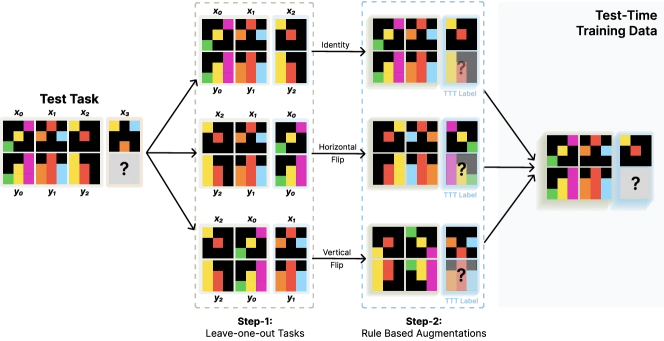
Figure 3 of Akyürek et al. 2024 (arXiv:2411.07279), reproduced for editorial coverage. Removing in-context format or geometric augmentation each roughly halves the TTT gain.

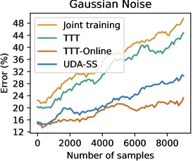
Figure 3 of Sun et al. 2020 (arXiv:1909.13231), reproduced for editorial coverage. Online TTT adapts across a stream of progressively-shifted inputs.

Hyperparameter sensitivity

Sun et al.: stable over $T \in [5, 20]$, $\eta \in [5 \times 10^{-4}, 5 \times 10^{-3}]$. Akyürek et al.: rank above 64, LR $5 \times 10^{-5}$ to $10^{-4}$, 2 epochs is a stable region; outside that range either underfits or overfits.

Robustness / stress tests

Sun et al. test on CIFAR-10.1 (unknown shift) and VID-Robust (gradual shift in video), reporting improvements in both. The CIFAR-10.1 result is the first published improvement on this benchmark: joint training error 16.7%, TTT 15.9%. ¹

Qualitative results

Sun et al. show a CIFAR-10-C grid of corrupted images with main-task confidence before and after TTT; the post-TTT confidence concentrates on the correct class. Akyürek et al. (Figure 1 right) show a representative ARC task that the fine-tuned LM fails on without TTT and solves with TTT, illustrating the kind of structural novelty TTT recovers.

Experimental scope limits

Sun et al.: vision only, ResNet-26 only, four-rotation auxiliary only. Subsequent work (Gandelsman et al. 2022 with masked autoencoders) extends the auxiliary choice; the original paper does not test transformer backbones. ⁶

Akyürek et al.: ARC only, Llama-family LMs only, LoRA rank up to 128 only. No test on natural-language reasoning benchmarks beyond ARC and a smaller BBH experiment (BIG-Bench Hard 10-shot reports $50.5\% \to 57.8\%$ via TTT, a 7.3 percentage-point gain). ⁴

Independent benchmark cross-checks for SOTA claims

[Analysis] Both papers’ SOTA-claims should be hedged carefully. Sun et al. is from 2020; the CIFAR-10-C and ImageNet-C numbers have since been superseded by various augmentation-heavy and transformer-based methods. The contribution that has aged well is the technique, not the absolute leaderboard position. Akyürek et al.’s ARC result is published outside the official ARC leaderboard compute budget; an independent reproduction is the open-source marc repository (Akyürek’s own GitHub), which the publication treats as author-side rather than independent. ¹⁸ [Reviewer Perspective] A fully-independent reproduction of the ARC TTT result has not yet been published as of 2026-05-20; the strongest independent signal is that the BARC component the authors ensemble with is itself an independently-developed system that performs in a similar accuracy band. ¹¹

Evidence audit

[Analysis] Strongly supported claims: (i) Sun et al.’s gradient-correlation theorem and its empirical verification on CIFAR-10-C ($r = 0.93$); (ii) the standard-TTT versus joint-training error gap (1.3 percentage points on CIFAR-10-C level 5) is a real, replicated isolation of the test-time-update contribution; (iii) Akyürek et al.’s ablation showing in-context format and geometric augmentation are jointly necessary for the ARC result.

Partially supported claims: the online TTT improvements on CIFAR-10-C are large (10.8 points) but the gain over standard TTT comes partly from non-stationary adaptation that the paper acknowledges may not replicate in deployment where test streams are reshuffled. The Akyürek et al. headline 6$\times$ accuracy gain depends on the choice of baseline (1B without TTT $\approx 5\%$ versus 1B + TTT $\approx 29\%$); against the 8B baseline the multiplier is smaller.

Claims relying on narrow evidence: extension to natural-language reasoning beyond ARC is supported only by a small BBH experiment in Akyürek et al.; no extended evaluation across MATH, GSM8K, or open-domain QA is reported.

Section 10: Technical novelty summary

Component	Type	Novelty level	Justification	Source
Per-sample test-time parameter update	Concept	Fully novel (Sun et al.)	Prior work on domain adaptation required batches; TTT operates on single samples	Sun et al. Section 3
Y-shaped multi-task architecture for TTT	Architecture	Incrementally novel	Multi-task architectures are standard; the specific use to enable per-sample test-time updates is the novelty	Sun et al. Section 3.1
Gradient-correlation theorem (Theorem 1)	Theory	Fully novel	First formal condition under which TTT provably improves main loss	Sun et al. Section 3.3
Rotation prediction as auxiliary	Method	Adopted	From Gidaris et al. 2018 self-supervised rotation pretraining	Sun et al. Section 3.2
Online TTT variant	Method	Incrementally novel	Sequential adaptation across a test stream; extends Standard TTT trivially	Sun et al. Section 3.4
Per-task LoRA TTT	Method	Combination novel	LoRA (adopted from Hu et al. 2021) used per-test-instance instead of as a global fine-tune	Akyürek et al. Section 3
Leave-one-out + invertible augmentation for ARC	Method	Fully novel	Specific construction not previously published for ARC TTT	Akyürek et al. Section 3.1
Hierarchical voting across augmentations	Method	Incrementally novel	Majority-vote-with-augmentation is standard; the two-stage scheme is the specific innovation	Akyürek et al. Section 3.3

Single most novel contribution. For Sun et al., the gradient-correlation theorem and its associated test-time update procedure, together they convert TTT from an empirical heuristic into a principled procedure with a checkable correctness condition. For Akyürek et al., the demonstration that LM TTT on ARC is competitive with average human performance when combined with program synthesis, a result that no fixed-weight approach has matched on ARC at the time of writing.

What the papers do NOT claim to be novel. Sun et al. do not claim novelty for joint multi-task training, rotation prediction as an auxiliary, or ResNet architecture. Akyürek et al. do not claim novelty for LoRA, AdamW, or the ARC benchmark itself; they explicitly position their ensemble pipeline as combining BARC’s program-synthesis component with their neural component. ^{4 11}

Section 11: Situating the work

What prior work did.

• Domain adaptation (DANN, CDAN, UDA-SS, etc.) assumed a batch of target-domain samples and explicit knowledge of the shift. Operated by aligning source and target features through adversarial training or feature matching. ¹
• Self-supervised pretraining (rotation prediction, Jigsaw, contrastive learning) used auxiliary tasks at pretraining to learn useful features. The features then froze at deployment. ¹⁴
• Robust training (AugMix, AutoAugment) used heavy training-time augmentation to expand the training distribution. Did not adapt to specific test inputs.

For LM reasoning, prior work was dominated by chain-of-thought prompting and self-consistency sampling (Wang et al. 2022) and, more recently, verifier-guided search (Snell et al. 2024). None updated weights at inference. ^{15 16}

What these papers change conceptually. Sun et al. introduce the per-sample parameter setting framing: $\theta(x)$ rather than fixed $\theta$. This is a small notational change with large consequences, it makes inference a small optimisation problem rather than a forward pass. Akyürek et al. demonstrate that this framing transfers to language-model reasoning, where the auxiliary loss is the in-context demonstration loss rather than a visual self-supervised task.

Cite at least 2 contemporaneous related papers. Gandelsman, Sun, Chen, Efros 2022 (“Test-Time Training with Masked Autoencoders”) extends Sun et al. by replacing rotation with masked-autoencoder reconstruction, achieving stronger results on ImageNet-C; the technical relationship is “same TTT framework, different auxiliary task.” ⁶ Sun, Li, Dalal, Xu, Vikram et al. 2024 (“Learning to (Learn at Test Time): RNNs with Expressive Hidden States”) reframes the hidden state of an RNN as a per-token TTT optimiser, making TTT continuous-time rather than discrete-per-sample; the technical relationship is “TTT as the inner-loop of a recurrent model.” ⁷ For the LM side, BARC (Li et al. 2024) is the strongest contemporaneous related work on ARC; Akyürek et al. ensemble explicitly with BARC’s program synthesiser. ¹¹ Tent (Wang et al. 2021) is the contemporaneous fully-test-time adaptation method that uses entropy minimisation as the self-supervised signal and updates only batch-norm statistics. ⁸

[Reviewer Perspective] Strongest skeptical objection. Sun et al.’s improvements are large only on corruptions where rotation prediction remains well-defined and informative; if a corruption breaks rotation prediction itself, TTT degrades. The paper does not test adversarial corruptions designed to fool rotation prediction, which would isolate the worst-case behaviour of TTT. For Akyürek et al., the 12-hour A100 cost per 100 tasks is a deployment-killer for any real-time application; the published improvements are at compute scales that exceed the official ARC leaderboard’s budget by more than an order of magnitude. ⁴

[Reviewer Perspective] Strongest author-side rebuttal grounded in the paper. Sun et al. address the auxiliary-task-degradation case by reporting the gradient-correlation diagnostic ($r = 0.93$) on the corruptions they test; the diagnostic generalises to any new corruption, measure the correlation on a small held-out set before deploying. Akyürek et al. note that compute cost is a function of LoRA rank and augmentation count; the recipe is presented as a recipe, not a deployment-optimised system, and a lower-cost variant (rank 32, fewer augmentations) achieves a smaller but still material gain.

What remains unsolved. When and why does the gradient-correlation condition hold for transformer architectures? Sun et al.’s theory assumes convexity. The empirical $r = 0.93$ on ResNet-26 is encouraging but does not generalise a priori to transformers, Sun et al. 2024 (“Learning to Learn at Test Time”) begins to address this in the RNN case but the transformer case is still an open question. ⁷

Three future research directions, each grounded in a paper-specific limitation.

• [Analysis] Replace LoRA-per-task in Akyürek et al. with a meta-learned initialisation that lets the per-task TTT converge in fewer steps. Current 12-hour-per-100-tasks compute is the deployment bottleneck; meta-learning the initialisation could plausibly reduce per-task TTT to seconds rather than minutes.
• [Analysis] Combine TTT with verifier-guided search (Snell et al. 2024). Both spend compute at inference; the former updates weights and the latter searches over completions. They are technically orthogonal and [Analysis] jointly applying them is an unexplored direction. ¹⁵
• [Reviewer Perspective] Investigate the failure modes of TTT under adversarial corruption. The gradient-correlation diagnostic could itself be attacked, an adversary who knows the auxiliary task could craft inputs where $r$ is high on the diagnostic but the post-TTT predictions are systematically wrong.

Section 12: Critical analysis

Strengths with concrete evidence. Sun et al.: a rare paper with both a clean theoretical result (Theorem 1, gradient-correlation guarantee) and strong empirical validation across multiple benchmarks (CIFAR-10-C average error reduction of 6.7 points; ImageNet-C improvements on all corruption types; first improvement on CIFAR-10.1). The Pearson $r = 0.93$ correlation between predicted and actual main-task improvement is unusually high for a deep-learning paper. Akyürek et al.: the ARC result is qualitatively striking, a benchmark designed to resist statistical pattern-matching, where the 8B model goes from 36% to 47% via test-time-only adaptation. ^{1 4}

Weaknesses explicitly stated by the authors. Sun et al. acknowledge in their conclusion that the convexity assumption in Theorem 1 does not hold for deep networks and that the result should be interpreted as a local-linearisation argument. They also note that the online variant assumes stationarity within a window, which can fail under sharp distribution shifts. Akyürek et al. acknowledge that the 12-hour-per-100-tasks A100 cost disqualifies their submission from the official ARC leaderboard, and that the BBH extension is preliminary. ^{1 4}

Weaknesses not stated by the authors. [Reviewer Perspective] Sun et al. do not explicitly compare against TENT (Wang et al. 2021), which is contemporaneous and reaches similar CIFAR-10-C numbers via a much simpler test-time update (only batch-norm statistics, not full trunk). The TTT vs. TENT comparison is a load-bearing one for the practical-deployment story and the absence is a real gap. ⁸ Akyürek et al. do not isolate the contribution of per-task LoRA versus the leave-one-out + augmentation construction; the headline number bundles both contributions and the ablation in Figure 3 does not fully separate them.

Reproducibility check.

• Sun et al. code: released, https://github.com/yueatsprograms/ttt_cifar_release (the publication has not independently verified the link state in 2026-05-20). The paper cites this repository in its abstract and Section 4.
• Sun et al. data: CIFAR-10-C, ImageNet-C, CIFAR-10.1, VID-Robust are all publicly released benchmarks.
• Sun et al. hyperparameters: fully reported in Section 4.1.
• Sun et al. compute: the paper reports inner-loop step counts but not wall-clock time; for ResNet-26 on a single GPU the cost is modest.
• Akyürek et al. code: released as ekinakyurek/marc on GitHub. ¹⁸
• Akyürek et al. data: ARC public validation is publicly released; the synthetic training mixtures (ReARC + LLM-generated tasks + BARC mixture) are released under the BARC repository. ¹¹
• Akyürek et al. hyperparameters: fully reported in Section 3 and Appendix B.
• Akyürek et al. compute: explicitly reported as $\sim 12$ hours on a single NVIDIA A100 for 100 tasks.
• Trained model weights: Sun et al. release ResNet-26 checkpoints; Akyürek et al. release fine-tuned base LM weights via Hugging Face.
• Evaluation set: ARC public validation is publicly accessible. The 80-task development subset is listed in the paper’s Table 2.
• Overall: both papers are fully reproducible in the sense that all code, data, hyperparameters, and compute requirements are published.

Methodology.

• Sample size: Sun et al., all 15 CIFAR-10-C corruption types at level 5 (10,000 test images each); ImageNet-C similar; CIFAR-10.1 2,000 images; VID-Robust 1,109 video frames. Akyürek et al., 80-task development subset for ablations, 400-task public ARC validation for headline numbers.
• Evaluation set: CIFAR-10-C / ImageNet-C / CIFAR-10.1 / VID-Robust are held-out from training. ARC public validation is held out from ARC training. No contamination check is reported in either paper but the benchmark structure makes contamination unlikely.
• Baselines: Sun et al., supervised ResNet-26, joint-trained ResNet-26 (same architecture, joint loss, no TTT), UDA-SS, several other UDA methods. Akyürek et al., fine-tuned LM without TTT at 1B and 8B sizes, BARC neural component alone, BARC program synthesiser alone, BARC + BARC synthesiser ensemble.
• Hardware/compute: Sun et al. do not explicitly report hardware in the main text. Akyürek et al. explicitly report single NVIDIA A100, with $\sim 12$ hours per 100 ARC tasks.

Generalisability.

[Analysis] Sun et al.’s framework generalises to any (main task, auxiliary task) pair where joint training shapes a shared trunk and the auxiliary task gradient correlates with the main task gradient. The principle has been extended to MAE-based auxiliary (Gandelsman et al. 2022), RNN hidden states (Sun et al. 2024), and policy adaptation in RL (Hansen et al. 2021). ^{6 7 9} Akyürek et al.’s framework generalises to any few-shot benchmark where (a) demonstrations carry enough signal for an adapter to specialise and (b) invertible augmentations exist. Non-grid reasoning benchmarks need a different augmentation design.

Assumption audit (revisiting Section 3 assumptions). The gradient-correlation assumption is checkable empirically, Sun et al.’s diagnostic should be run on any new (main task, auxiliary task) pair before deployment. The “invertible augmentation” assumption in Akyürek et al. is benchmark-specific and is the hardest to port to non-grid reasoning.

What would make the papers significantly stronger. [Analysis] Sun et al.: a head-to-head comparison with TENT, plus an evaluation on transformer backbones. Akyürek et al.: an ablation that fully isolates per-task LoRA from leave-one-out from invertible augmentation, plus a fully-independent reproduction. A meta-learned initialisation for the per-task LoRA would also address the deployment-cost objection.

Section 13: What is reusable for a new study

REUSABLE COMPONENT 1: Y-shaped multi-task architecture for TTT.

• What it is: shared trunk + main head + self-supervised head, jointly trained.
• Why worth reusing: the joint-training pressure shapes the trunk to support both heads, which is the precondition for TTT to work.
• Preconditions: an auxiliary task whose gradient correlates with the main task gradient at the trunk’s parameter setting.
• What would need to change in a different setting: the choice of auxiliary task. For transformers and language models, masked-token prediction or next-token-on-demos replaces rotation.
• Risks: if the auxiliary task is too easy, the trunk collapses to the auxiliary task and main-task performance degrades.
• Interaction effects: joint training cost is approximately equal to single-task training cost because the auxiliary head is small.

REUSABLE COMPONENT 2: Gradient-correlation diagnostic.

• What it is: measure $\text{corr}(\langle \nabla \ell_m, \nabla \ell_s \rangle, \Delta \ell_m)$ on a held-out validation set before deploying TTT.
• Why worth reusing: it’s the only known way to predict TTT effectiveness without running the full experiment.
• Preconditions: a held-out set with main-task labels.
• What would need to change: the gradient computation cost scales with $\mid \theta_e\mid$; for very large models, low-rank approximations may be needed.
• Risks: high correlation on the diagnostic does not guarantee correlation on the deployment distribution.
• Interaction effects: the diagnostic is cheap relative to full TTT evaluation.

REUSABLE COMPONENT 3: Per-task LoRA with leave-one-out + invertible augmentation.

• What it is: for each test instance, build a synthetic training set via leave-one-out on demonstrations and invertible augmentations, train a fresh LoRA adapter for 2 epochs, predict with the adapter under augmentations, vote.
• Why worth reusing: the construction is benchmark-agnostic in its outline; only the augmentation set is benchmark-specific.
• Preconditions: a few-shot benchmark with structured demonstrations and a base model that has been fine-tuned on the demonstration format.
• What would need to change: the augmentation set. For natural-language reasoning, semantic-preserving paraphrases could substitute for geometric augmentations.
• Risks: compute cost. Per-task LoRA at rank 128 with 2 epochs of augmented data is expensive at deployment.
• Interaction effects: the technique composes with chain-of-thought (the model can still produce CoT tokens within the LoRA-adapted forward pass) and with self-consistency (CoT sampling can happen at the augmented-inference stage).

REUSABLE COMPONENT 4: Hierarchical voting across invertible augmentations.

• What it is: two-stage majority vote, top-3 within each augmentation, top-2 across augmentations, with identity-transformation tiebreak.
• Why worth reusing: the scheme is robust to outliers in individual augmentations and approaches oracle accuracy on ARC.
• Preconditions: invertible augmentations.
• What would need to change: tiebreak heuristic if the application has no analogue of “identity transformation.”
• Risks: requires running multiple inferences; cost scales with augmentation count.
• Interaction effects: combines naturally with self-consistency sampling at the per-augmentation level.

Dependency map. Component 1 (Y-shape) is the training-time foundation; Component 2 (correlation diagnostic) is the deployment-time check that uses the trained Y-shape. Component 3 (per-task LoRA) is independent of Components 1-2, it can apply to a pretrained LM with no Y-shape, using in-context-demonstration loss as the self-supervised signal. Component 4 (hierarchical voting) is downstream of Component 3 in the LM pipeline; it does not apply to Sun et al.’s vision setting.

Recommendation: highest-value components. [Analysis] For a vision robustness deployment, Components 1 and 2 are the highest-value pair, they implement TTT directly. For an LM few-shot reasoning deployment, Component 3 is the headline; Component 4 is a 5-10 percentage-point booster on top of Component 3 per the Akyürek et al. ablation.

[Analysis] What type of new study benefits most: studies on (a) vision robustness with per-sample shifts, (b) LM few-shot benchmarks with structured demonstrations, (c) any “test-time compute” line of research that has so far been restricted to fixed-weight techniques like CoT and self-consistency.

Section 14: Known limitations and open problems

Limitations explicitly stated by the authors.

• Sun et al.: convexity assumption in Theorem 1 does not hold for deep networks; online variant assumes within-stream stationarity that fails under sharp shifts.
• Akyürek et al.: 12-hour per-100-tasks compute cost; restricted scope to ARC and a small BBH experiment; ensemble with BARC means the headline number is not pure TTT.

Limitations not stated by the authors. [Reviewer Perspective] Sun et al. omit a TENT baseline (Wang et al. 2021), which is the contemporaneous fully-test-time adaptation method and reaches similar CIFAR-10-C numbers via a simpler update. ⁸ Akyürek et al. do not separately ablate per-task LoRA versus leave-one-out versus augmentation in a 2x2x2 design; the published ablation is one-at-a-time. The 6$\times$ accuracy multiplier is anchored on the 1B baseline; against the 8B baseline the multiplier is closer to 1.3$\times$. ⁴

Technical root causes.

• The convexity gap in Sun et al.’s theorem: deep networks have non-convex loss landscapes; the theorem is best interpreted as a local first-order argument valid in a small neighbourhood. Extending to a non-convex bound is open.
• The compute cost in Akyürek et al.: dominated by 2 epochs of LoRA training over $\sim 200$ synthetic examples per test instance. A meta-learned LoRA initialisation could plausibly bring this to 1 epoch or fewer; this is the open follow-up direction.
• The TENT-vs-TTT gap in Sun et al.: not addressed in the paper. Likely candidates for closure: a benchmark-by-benchmark head-to-head, plus a unified analysis that places both methods in a single framework (parameter subset to update, choice of test-time loss).

Open problems left behind. (i) Meta-learned TTT initialisations. (ii) TTT on transformer backbones with full attention parameter updates. (iii) Adversarial robustness of TTT itself. (iv) Joint TTT + verifier-guided search for LM reasoning. (v) Theoretical analysis of TTT in non-convex regimes.

What a follow-up paper would need to solve to address the most critical limitation. For Sun et al., the most critical limitation is the convexity-assumption gap; closing it would require either a PL-condition-style relaxation or a fully empirical guarantee over a sufficiently rich function class. For Akyürek et al., the most critical limitation is the 12-hour compute cost; closing it requires either a meta-learned initialisation that converges in 1-2 gradient steps, or a way to amortise the per-task LoRA across multiple test instances of the same task family.

How this article reads at three depths

For the curious high-school reader. Most machine-learning models freeze their weights once training finishes and then use those frozen weights to answer every question. Test-time training breaks that rule: when a hard question shows up at inference, the model briefly retrains itself on that one question using a side-task that doesn’t need a correct answer to learn from. Sun et al. showed this works for image classification when images are noisy or corrupted, and Akyürek et al. showed it works for language models on hard reasoning puzzles. The trick takes more compute at inference, but it lets models solve problems that fixed-weight models cannot.

For the working developer or ML engineer. TTT is a third axis of test-time compute alongside chain-of-thought (more tokens) and reinforcement fine-tuning (training-time adjustment for inference-time reasoning). Sun et al.’s Y-shaped network with rotation auxiliary is the canonical recipe for vision robustness, with a checkable gradient-correlation diagnostic that predicts when TTT will help. Akyürek et al.’s per-task LoRA recipe on ARC delivered a $36\% \to 47\%$ jump on an 8B fine-tuned LM at $\sim 7$ minutes per task on an A100, large gains, expensive deployment. The technique is worth investing engineering time on if (a) your test distribution has per-sample shifts, (b) you have a self-supervised auxiliary task whose gradient correlates with your main task, and (c) you can absorb a $10\times$ inference-cost multiplier. The technique is not worth investing in if you need sub-second latency or your test distribution is well-covered by training augmentations.

For the ML researcher. The Sun et al. gradient-correlation theorem is the load-bearing theoretical contribution, a convex one-step guarantee plus an empirical $r = 0.93$ correlation between $\langle \nabla \ell_m, \nabla \ell_s \rangle$ and observed main-task improvement. The convexity assumption is the obvious gap; an extension to PL-condition or non-convex bounds is the open follow-up. Akyürek et al.’s per-task LoRA construction is novel in combination but each ingredient (LoRA, leave-one-out, invertible augmentation, hierarchical voting) is [Adopted] or [Adapted] individually; the ablation does not fully isolate the contributions. The strongest objection to the Akyürek et al. ARC result is the 12-hour-per-100-tasks compute cost, which exceeds the official ARC leaderboard budget by more than an order of magnitude. A follow-up that meta-learns the per-task LoRA initialisation to converge in $\leq 2$ steps would be decisive. The under-explored research direction the publication’s reading flags is the joint composition of TTT with verifier-guided search (Snell et al. 2024), both spend inference compute but on orthogonal axes, and the combination has not been published.