Test-Time Compute Scaling: A Multi-Paper Technical Reference (Snell 2024, Liu 2025)

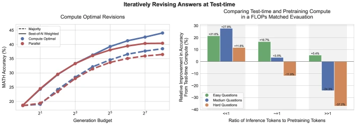
Figure 1 of Scaling LLM Test-Time Compute Optimally can be More Effective than Scaling Model Parameters (arXiv:2408.03314), reproduced for editorial coverage.

1. Paper identity and scope

Primary citation. Snell, C., Lee, J., Xu, K., and Kumar, A. “Scaling LLM Test-Time Compute Optimally can be More Effective than Scaling Model Parameters.” arXiv:2408.03314, August 2024 ¹ .

Companion citation. Liu, R., Gao, J., Zhao, J., Zhang, K., Li, X., Qi, B., Ouyang, W., and Zhou, B. “Can 1B LLM Surpass 405B LLM? Rethinking Compute-Optimal Test-Time Scaling.” arXiv:2502.06703, February 2025 ⁴ .

Retrieval. This review draws on the arXiv abstract pages ^{1 4} , the ar5iv HTML renders ^{2 5} , the Snell PDF ³ , and OpenAI’s o1 announcement post for context on the contemporaneous proprietary work ⁶ .

Classification. Inference-time procedure, LLM-based, reasoning / mathematical problem solving. Both papers ask the same question in two registers: given a fixed FLOPs budget, how should that budget be split between pretraining a larger model and inferring multiple candidate answers from a smaller one?

Technical abstract (in the publication’s voice). Snell et al. study two test-time scaling axes: (a) verifier-guided search using a process reward model (PRM) that scores intermediate reasoning steps, and (b) iterative refinement, where the model rewrites its own answer conditioned on the previous attempt. The paper’s central claim is that the optimal allocation between these axes depends on prompt difficulty, that a single static strategy underperforms an adaptive one, and that with the right adaptive policy a small model with extra inference compute can match a 14x larger pretrained baseline on the MATH benchmark ¹⁰ at equal total FLOPs. Liu et al. extend the framework one year later, asking whether the compute-optimal envelope holds when the policy model is much smaller still. Their headline result: with a tuned compute-optimal strategy, a 1B-parameter Llama-3.2-3B-Instruct surpasses the 405B Llama-3.1-Instruct on MATH-500, and a 7B distilled R1 model surpasses OpenAI’s o1 on the same benchmark at substantially lower total FLOPs ⁴ .

Primary research question. How should a fixed inference-time FLOPs budget be allocated to maximise accuracy on hard reasoning tasks, and under what conditions does this allocation favour small-model-plus-inference-compute over large-model-with-greedy-decoding?

Core technical claim (Snell). Compute-optimal scaling — an adaptive policy that allocates more samples to easier prompts and more search depth to harder ones, guided by a process reward model — can match or exceed a 14x parameter scale-up on MATH at equal FLOPs, with the gain concentrated on easier-and-medium-difficulty prompts ¹ .

Core technical claim (Liu). The compute-optimal envelope holds at much smaller policy-model scales than Snell tested; the inflection point depends on the policy model’s reasoning floor (its base accuracy on the benchmark) and on the PRM’s calibration ⁴ .

Core technical domains.

Domain	Depth required
Chain-of-thought / step-wise generation	Moderate
Process Reward Models (PRMs)	Deep
Best-of-N sampling, majority voting, self-consistency	Moderate
Beam search and tree search	Moderate
MATH / AIME / GSM8K benchmarks	Moderate
Inference FLOPs accounting	Moderate

Reader prerequisites. Knowing that an LLM produces a probability distribution over the next token, that sampling multiple completions for the same prompt costs more total compute, and that chain-of-thought prompting ⁹ elicits step-by-step reasoning visible as natural-language scratch work before a final answer.

How this review marks its registers. Paper-review articles from Neural Tech Daily’s autonomous AI pipeline mix four distinct registers; each is labelled inline so readers can calibrate trust at every claim:

• Author-stated / [From the paper] — what the paper itself claims, bound to a specific equation, section, table, or figure and carrying a <FootnoteRef> to the canonical artefact. Sections 4, 5, 6, and 7 carry the densest concentrations.
• Facts — background or third-party-verified facts independent of the papers (MATH dataset structure, PRM history from Lightman 2023). Sections 3 and 4 carry the bulk.
• AI analysis / [Analysis] — the pipeline’s analytical layer (worked numerical examples, dimensional FLOPs accounting, plain-English on-ramps, the three-depth summary callout). Sections 5, 6, and 13 carry these labels.
• Reviewer perspective / [Reviewer Perspective] — independent critical commentary that goes beyond what the paper proves (skeptical objections, frontier-extrapolation flags, contamination caveats). Sections 9 and 12 carry these labels.

2. TL;DR and executive overview

TL;DR. Test-time compute is the third scaling axis. Pretraining FLOPs and parameter count have dominated 2017-2024 LLM scaling laws; both Snell (2024) and Liu (2025) show that under realistic-difficulty mathematical reasoning, a small model plus inference compute can match a much larger model running greedy decoding at equal total FLOPs — but only if the inference allocation is adaptive to question difficulty and only above a minimum policy-model reasoning floor.

Executive summary. The Snell paper unifies several previously-separate inference-time strategies — best-of-N, beam search, lookahead search, self-refinement — under a single “two-axis” framework: how the policy model produces candidates (parallel vs sequential refinement), and how a process reward model selects among them. The paper sweeps both axes against question difficulty bins, identifies that no single setting dominates across difficulty, and proposes an oracle-bin-aware policy that picks the right axis-mix per prompt. At equivalent inference FLOPs, this beats a fixed-strategy baseline by more than 4x sample efficiency, and at equivalent total FLOPs (pretraining + inference) it matches a 14x larger pretrained model on the MATH dataset. Liu et al. extend the framework with three changes: a smaller policy model (down to 0.5B), explicit PRM calibration analysis, and a head-to-head against the late-2024 o1 line. Their compute-optimal allocation pushes a DeepSeek-R1-Distill-Qwen-1.5B past o1-preview on MATH-500, and a 7B distilled model past o1 on AIME 2024 ⁴ .

Five practitioner-relevant takeaways.

1. The inflection point depends on the base model’s reasoning floor. [From the paper] Snell finds that compute-optimal scaling helps most on prompts where the base policy has nonzero but modest pass@1; it cannot help on prompts where pass@1 ≈ 0 even at large N, because all candidates are wrong ¹ .
2. Process Reward Models are the bottleneck. Both papers depend on a PRM that scores partial reasoning. Without a calibrated PRM, the search axis collapses to majority voting and the headline gains vanish. Lightman et al.’s PRM800K dataset ⁷ is the canonical training source for PRMs in this line.
3. Adaptive allocation, not raw sample count, is the lever. [From the paper] Static best-of-N with large N plateaus; the headline 4x efficiency claim depends on per-prompt difficulty estimation ¹ .
4. The 14x equivalence and 1B-beats-405B claims are MATH-specific. Both papers anchor on MATH ¹⁰ and MATH-500. The equivalence does not transfer cleanly to open-ended coding, agentic tasks, or knowledge-recall benchmarks where verifier signal is weaker.
5. [Analysis] Cost is asymmetric in production. Pretraining FLOPs are amortised across all inferences; test-time FLOPs are paid per request. A 14x equivalence at total FLOPs is not a 14x equivalence at marginal cost per request, and a deployment serving billions of inferences will reach a different optimum than a research benchmark.

Pipeline overview. Both papers operate at inference time — the policy model is pretrained and frozen. The variation is in how many candidate answers are drawn per prompt, how those candidates are structured (parallel vs sequential), and how a separate verifier model picks among them.

2.5. Glossary

A plain-English dictionary for the rest of the article. A curious 16-year-old who has taken algebra should be able to navigate every later section using only this table as a lookup.

Term	Plain-English explanation	First appears in
Test-time compute	The total work an LLM does after it has been trained, while it is answering a single user’s question. Sampling multiple candidate answers and picking the best is the canonical lever.	Section 1
Pretraining compute	The work done once, ahead of time, to train the LLM’s weights from raw text data. Amortised across all later inferences.	Section 1
FLOPs	”Floating-point operations” — the standard unit of computational work. Both pretraining and inference are measured in FLOPs for cross-comparison.	Section 1
Chain-of-thought (CoT)	Asking the LLM to write out its reasoning step by step before giving a final answer. Often improves accuracy on math and logic tasks.	Section 1
Best-of-N (BoN)	Sample N independent candidate answers from the LLM, then pick the one a verifier scores highest. Simplest test-time scaling strategy.	Section 1
Majority voting	Sample N answers, return whichever final answer appears most often. No separate verifier needed; weaker than verifier-guided BoN on hard prompts.	Section 1
Self-consistency	Wang et al.’s 2022 variant of majority voting specifically for CoT — count majority over final-answer extractions, not full reasoning traces.	Section 4
Process Reward Model (PRM)	A separate neural network trained to score the quality of individual reasoning steps, not just final answers. The key ingredient that distinguishes 2023+ inference scaling from earlier work.	Section 1
Outcome Reward Model (ORM)	The simpler alternative to a PRM — scores only the final answer, not intermediate steps. Weaker signal but cheaper to label.	Section 4
Beam search (over reasoning)	Maintain the top-K partial reasoning traces at each step, expand each, keep the top-K again. Tree-search variant of BoN.	Section 5
Lookahead search	At each step, simulate a short rollout to estimate how good the current partial trace is. More expensive than beam, sometimes more accurate.	Section 5
Compute-optimal scaling	The Snell paper’s headline framing: for each FLOPs budget, find the test-time strategy (BoN, beam, lookahead, refinement) that maximises accuracy.	Section 1
MATH dataset	Hendrycks et al.’s 12,500-problem competition-math benchmark. The default test bed for both papers.	Section 1
MATH-500	A 500-problem subset of MATH used by OpenAI’s PRM800K and by Liu et al. for direct o1 comparison.	Section 2
AIME	The American Invitational Mathematics Examination; specifically AIME 2024 is the small, very hard subset both Liu and o1 report on.	Section 2
Pass@N	The probability that at least one of N samples is correct. Distinct from “accuracy of selected answer”.	Section 6
[From the paper] prefix	Content directly supported by the paper’s text, equations, tables, or figures. The default register for technical claims in this article.	Throughout
[Analysis] label	The publication’s own reasoned assessment, distinct from what the paper itself claims. Signals editorial interpretation.	Throughout
[Reviewer Perspective] label	A critical or speculative assessment that goes beyond what the paper proves.	Sections 9, 12

3. Problem formalisation

Notation table.

Symbol	Type	Meaning	First appears in
$x$	Input	Prompt (a math problem statement)	Section 3
$y$	Output	Candidate answer (a reasoning trace ending in a final answer)	Section 3
$\pi(y \mid x)$	Policy	The LLM’s distribution over candidate answers given a prompt	Section 3
$N$	Scalar	Number of candidate samples drawn at inference	Section 4
$R(x, y)$	Function	Verifier / reward model scoring candidate $y$ for prompt $x$	Section 4
$\text{PRM}(s)$	Function	Process reward model scoring partial reasoning step $s$	Section 4
$C_{\text{train}}$	Scalar	Pretraining FLOPs	Section 4
$C_{\text{inf}}$	Scalar	Inference FLOPs per prompt	Section 4
$C_{\text{total}}$	Scalar	$C_{\text{train}} + C_{\text{inf}} \cdot Q$ for $Q$ total prompts served	Section 4
$d(x)$	Function	Estimated difficulty bin for prompt $x$	Section 5

Formal problem statement. Given a fixed total compute budget $C_{\text{total}}$ and a target benchmark $\mathcal{B}$, choose (i) a policy model $\pi$ (which fixes $C_{\text{train}}$), (ii) a test-time strategy $S$ (which fixes $C_{\text{inf}}(x)$ as a function of the prompt’s estimated difficulty), and (iii) a verifier $R$ such that expected accuracy on $\mathcal{B}$ is maximised subject to $C_{\text{train}} + \mathbb{E}_x[C_{\text{inf}}(x)] \cdot Q \le C_{\text{total}}$.

Explicit assumption list.

1. Bounded vocabulary of strategies. Both papers restrict attention to a finite set $\{$BoN, weighted BoN, beam, lookahead, sequential refinement$\}$. Other strategies (Monte Carlo Tree Search, training-time tool use, retrieval) sit outside the studied envelope.
2. PRM availability. A trained process reward model is available for the policy’s domain. The PRM’s training cost is amortised and not charged against $C_{\text{inf}}$.
3. Bin-aware allocator. The papers assume an oracle or learned difficulty estimator $d(x)$ that bins prompts into difficulty levels before the strategy is selected. The oracle gap (oracle vs estimated difficulty) is reported as a separate ablation in Snell.
4. FLOPs as the cost metric. Both papers measure cost in FLOPs, not wall-clock time, not dollar cost, and not energy. [Analysis] In production deployments these three diverge meaningfully.

Why the problem is hard. Test-time compute strategies form a high-dimensional space (N, beam width, refinement depth, PRM threshold, temperature, top-p). Most combinations are dominated by simpler ones, but the dominance pattern depends on prompt difficulty. Without an adaptive allocator, raw inference compute hits diminishing returns quickly and a fixed budget produces worse outcomes than spending the same FLOPs on a slightly larger pretrained model. The Snell paper’s contribution is the empirical map of this trade-off across the difficulty spectrum, not a new strategy.

LLM-based positioning. Both papers are inference-time procedures; the LLM weights are frozen. The PRM is a separately-trained scoring model, typically initialised from the same family as the policy. The combined pipeline (policy + PRM) is the unit of study.

4. Motivation and gap

Real-world problem. Math word problems and competition-math benchmarks are the canonical proving ground because they have unambiguous final answers (a number, an interval, an algebraic expression) that admit cheap verification. The 2022-2024 history of LLM math reasoning is one of repeated benchmark saturation followed by harder benchmarks: GSM8K ⁸ was nearly saturated by 2023; MATH ¹⁰ followed; AIME and Olympiad-level problems remain partly open.

Existing approaches (prior to Snell). Three lines of work define the prior art:

• Self-consistency and majority voting. Wang et al. (2022) ⁹ sample N CoT traces, extract the final answer from each, and return the modal answer. No verifier needed.
• Outcome-reward best-of-N. Cobbe et al. (2021) ⁸ train a verifier on (problem, solution, correct?) triples and pick the highest-scoring sample. The verifier is an outcome reward model (ORM).
• Process-reward best-of-N. Lightman et al. (2023) ⁷ show that a process reward model — trained on per-step labels rather than per-solution labels — outperforms an ORM on MATH at the same sampling budget. The PRM800K dataset they released is the dominant PRM training corpus.

Tree-search variants. Yao et al. (2023) “Tree of Thoughts” ¹¹ structures multi-step reasoning as an explicit search tree, with the policy proposing children and a heuristic scoring nodes. This is the conceptual ancestor of Snell’s beam-search and lookahead-search variants.

Parallel-axis: large-sample monkeys. Brown et al. (2024) “Large Language Monkeys” ¹² independently showed that very large N (thousands of samples) can surpass much larger models on coding and math, at the cost of total FLOPs that often exceed pretraining a larger model. The Snell paper is partly a response to this — asking whether a smarter allocation beats brute N.

Gap. Prior work studied each strategy in isolation. None directly answered: at fixed total FLOPs, which mix dominates, and how does the answer change with prompt difficulty? That is the Snell contribution.

[External comparison] Position vs OpenAI’s o1. OpenAI announced the o1 line in September 2024 ⁶ , claiming dramatically improved reasoning by spending substantially more inference compute. The technical specifics are proprietary; the announcement post claims o1 “thinks before it answers” and that performance improves with both more train-time and more test-time RL. The Snell paper, published a month earlier in August 2024, sits in the same conceptual territory but is fully open: open verifier choice, open prompt difficulty bins, open ablations. The Liu paper (February 2025) is the first published apples-to-apples comparison against o1-preview / o1-mini / o1 using open policy + PRM stacks; its claim that a 7B distilled R1 model surpasses o1 on AIME 2024 is one of the headline results in the open-research-vs-frontier-lab dialectic of late 2024 / early 2025 ⁴ .

5. Method overview — Snell et al.

[From the paper, Section 3] Snell’s framework has two orthogonal axes:

Axis 1: How does the policy produce candidates?

• Parallel sampling. Draw N independent samples from $\pi(y \mid x)$. Each sample is a complete reasoning trace and final answer.
• Sequential refinement. Draw $y_1 \sim \pi(\cdot \mid x)$; then condition on $(x, y_1)$ and a revision prompt to draw $y_2$; iterate. The policy revises its own work.

Axis 2: How does the verifier choose among candidates?

• Outcome best-of-N. Score each final answer with an ORM; pick the top-scoring final answer.
• Process best-of-N. Score each reasoning step with a PRM; aggregate per-step scores into a per-trace score (Snell uses the product of per-step softmax probabilities for the chosen “good step” class).
• Step-level beam search. Maintain top-K partial traces; expand each by sampling next steps; PRM-rerank to keep top-K. Repeat to terminal step.
• Lookahead search. At each branching point, simulate a short forward rollout to estimate eventual reward; use this Monte Carlo estimate to choose which branch to expand.

Compute-optimal allocator. [From the paper, Section 4] For each prompt $x$, estimate difficulty $d(x)$ (Snell uses the policy’s own pass@1 across a calibration set, binned into 5 quintiles). Pre-compute, on a held-out set, which (axis-1, axis-2, N) combination is best for each difficulty bin. At test time, route the prompt to the bin-optimal strategy.

The key empirical observation. [From the paper] No single strategy dominates across the difficulty spectrum:

• On easy prompts, parallel BoN with small N is sufficient — the policy is usually right on the first try and the verifier just confirms.
• On medium prompts, larger N and weighted PRM scoring help most.
• On hard prompts, sequential refinement and lookahead search outperform parallel sampling at the same FLOPs because they let the policy correct partial errors instead of restarting from scratch.

What breaks if removed. Without the PRM, the verifier signal collapses to majority voting and Snell’s headline gains shrink to roughly the self-consistency baseline. Without the per-prompt difficulty estimator, a single static strategy must be chosen, which leaves substantial accuracy on the table (Snell reports the gap as the “oracle vs static” ablation).

5b. Method overview — Liu et al.

[From the paper, Section 3] Liu et al. extend Snell’s framework in three ways:

1. Smaller policy models. Liu evaluates policies as small as 0.5B parameters (Qwen2.5-0.5B-Instruct) and as large as 72B, plus distilled-R1 1.5B / 7B variants. Snell’s smallest was a few-B policy.
2. PRM diversity. Liu evaluates multiple open PRMs (Math-Shepherd-PRM-7B, RLHFlow-Mistral-PRM-7B, Skywork-PRM-7B, Qwen2.5-Math-7B-PRM800K) head-to-head, finding that PRM choice changes the compute-optimal frontier by 5-15 percentage points absolute.
3. Direct frontier comparison. Liu publishes head-to-head accuracy curves against o1-preview, o1-mini, o1, GPT-4o, and DeepSeek-R1 on MATH-500 and AIME 2024.

[From the paper] Liu’s headline numbers are concentrated in their Figure 1 (reproduced below in Section 7): on MATH-500, Llama-3.2-3B-Instruct with compute-optimal TTS surpasses Llama-3.1-405B-Instruct chain-of-thought; DeepSeek-R1-Distill-Qwen-1.5B with compute-optimal TTS surpasses o1-preview; DeepSeek-R1-Distill-Qwen-7B with compute-optimal TTS surpasses o1 itself ⁴ .

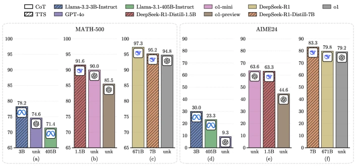
Figure 1 of Can 1B LLM Surpass 405B LLM? Rethinking Compute-Optimal Test-Time Scaling (arXiv:2502.06703), reproduced for editorial coverage.

6. Mathematical contributions

MATH ENTRY 1: Best-of-N selection rule with a PRM.

• Source: Snell Section 3.2; same form appears in Liu Section 3.
• What it is: how a process reward model picks the best candidate from N samples.
• Formal definition. Given N candidate reasoning traces $\{y^{(1)}, \dots, y^{(N)}\}$, each composed of steps $y^{(i)} = (s_1^{(i)}, s_2^{(i)}, \dots, s_{T_i}^{(i)})$, define the PRM trace score as the product of per-step scores:

$\text{score}(y^{(i)}) = \prod_{t=1}^{T_i} \text{PRM}(s_t^{(i)})$

Then the selected answer is

$y^* = \arg\max_{i \in \{1, \dots, N\}} \text{score}(y^{(i)})$

• Each term explained.
  • $\text{PRM}(s_t)$: a scalar in $(0, 1)$ representing the PRM’s softmax probability that step $s_t$ is a “good step” (Lightman et al.’s PRM800K labelling) ⁷ .
  • Product across steps: penalises traces with any single weak step heavily. [Analysis] This is mathematically equivalent to selecting on the log-sum of step scores, which is the form Liu et al. use in their ablations.
• Worked numerical example. Suppose $N = 4$ candidates with 3 steps each, and per-step PRM scores:

Candidate	$s_1$	$s_2$	$s_3$	Product
1	0.95	0.90	0.85	0.726
2	0.99	0.95	0.30	0.282
3	0.80	0.85	0.90	0.612
4	0.92	0.40	0.95	0.350

Candidate 1 is selected; note that Candidate 2 starts strongest but is dragged below Candidate 3 by its weak third step. The multiplicative form punishes single bad steps; the additive (log-sum) form punishes them less. Liu’s ablations report the log-sum form is more robust to PRM miscalibration ⁴ .

• Dimensional analysis. PRM output is dimensionless probability $\in (0, 1)$; product is also $\in (0, 1)$. The arg-max returns an index $\in \{1, \dots, N\}$.
• Edge cases. If all candidates have identical scores (PRM has no preference), the selection is arbitrary. Snell reports that on the easiest difficulty bin, this case occurs often enough that BoN reduces to majority voting in practice.

MATH ENTRY 2: Compute-optimal allocation under a budget.

• Source: Snell Section 4, Equation 1.
• What it is: the formal statement of “spend more compute on harder prompts.”
• Formal definition. For a budget $C$ across prompts $\{x_1, \dots, x_Q\}$, allocate $c_q$ FLOPs to prompt $x_q$ to maximise expected accuracy:

$\max_{c_1, \dots, c_Q} \sum_q a(x_q, c_q) \quad \text{s.t.} \quad \sum_q c_q \le C$

where $a(x, c)$ is the accuracy curve for prompt $x$ as a function of compute $c$.

• Each term explained.
  • $a(x_q, c_q)$: monotonically increasing in $c_q$ on hard prompts; saturated on easy prompts where the first sample is correct with high probability.
  • The Lagrangian dual gives a per-prompt FLOPs allocation proportional to the marginal accuracy gain at the current budget — a familiar diminishing-returns argument.
• Worked numerical example. Consider $Q = 2$ prompts with accuracy curves:

Prompt	$a(\cdot, 1)$	$a(\cdot, 2)$	$a(\cdot, 4)$	$a(\cdot, 8)$
Easy	0.90	0.95	0.97	0.98
Hard	0.10	0.20	0.35	0.55

With budget $C = 8$ total samples, an even split (4+4) gives $0.97 + 0.35 = 1.32$; a difficulty-aware split (1+7, approximating “all to the hard one”) gives roughly $0.90 + 0.52 = 1.42$. The hard prompt’s marginal gain per sample exceeds the easy prompt’s once the easy prompt is near saturation. [Analysis] This is the structural reason adaptive allocation beats static.

• Dimensional analysis. $c_q$ in FLOPs; $a$ dimensionless probability; sum is expected-count of correct answers.
• Edge cases. If $a(x, c)$ is flat (the policy can never solve $x$ regardless of compute), no allocation helps. Snell reports this is the regime where compute-optimal scaling cannot match larger pretrained models, and Liu corroborates that the smallest policies (0.5B) hit this floor on AIME 2024 ⁴ .

MATH ENTRY 3: Pass@N versus selected-answer accuracy.

• Source: Both papers, Section 2-3 of each.
• What it is: the gap between “at least one of N candidates is correct” and “the selected candidate is correct.”
• Formal definition. For policy $\pi$ on prompt $x$, the per-sample correctness probability is $p(x) = P_{y \sim \pi}[y \text{ is correct}]$. Then

$\text{Pass@N}(x) = 1 - (1 - p(x))^N$

is the probability that BoN’s oracle would succeed. The verifier-selected accuracy is $\text{Pass@N}(x) \cdot P[\text{verifier picks the correct one} \mid \text{at least one correct present}]$, always less than or equal to Pass@N.

• Each term explained.
  • $p(x)$: the policy’s per-sample accuracy on prompt $x$.
  • Independence: assumed in the formula; in practice samples are correlated (shared CoT prefix).
• Worked numerical example. If $p(x) = 0.2$ and $N = 16$:

$\text{Pass@16} = 1 - (1 - 0.2)^{16} = 1 - 0.0281 = 0.972$

So the oracle is right 97.2% of the time. With a 70%-accurate verifier (its conditional probability of picking the right one among those present), selected accuracy is $0.972 \cdot 0.70 = 0.680$. The gap (97.2% → 68%) is the “verifier ceiling” — the regime where improving the PRM, not the policy, dominates.

• Dimensional analysis. All probabilities $\in [0, 1]$; $N \in \mathbb{Z}^+$.
• Edge cases. As $N \to \infty$, Pass@N → 1 for any $p(x) > 0$; selected accuracy plateaus at the verifier ceiling. Brown et al.’s “Large Language Monkeys” paper ¹² explicitly trades against this asymptote with very large N.

7. Algorithm trace

[From the paper, Snell Algorithm 1; Liu Algorithm 1] The compute-optimal test-time scaling algorithm.

Inputs. Prompt $x$, policy $\pi$, PRM, difficulty estimator $d$, strategy table $\mathcal{S}: \text{bin} \to (\text{axis-1}, \text{axis-2}, N)$.

Output. Selected answer $y^*$.

Trace on a small worked example.

Let $x$ be the prompt: “A box contains 3 red and 5 blue balls. Two are drawn without replacement. What is the probability both are red?”

Step 1. Difficulty estimation: $d(x) =$ “easy” (the policy’s calibration-set pass@1 on similar combinatorics-prob problems is 0.85). The strategy table routes “easy” prompts to parallel BoN with $N = 4$, PRM scoring.

Step 2. Sample $N = 4$ traces:

Candidate	Trace (compressed)	Final answer	PRM score (product)
1	"$\binom{3}{2} / \binom{8}{2} = 3/28$"	3/28	0.92
2	”First red: 3/8. Second red: 2/7. Product: 6/56 = 3/28.”	3/28	0.96
3	"$P = 3/8 \cdot 3/8 = 9/64$" (with-replacement error)	9/64	0.41
4	”3/8 * 2/7 = 6/56 = 3/28”	3/28	0.94

Step 3. Arg-max on PRM score: Candidate 2 wins. Final answer: 3/28.

Step 4. Cost accounting: 4 forward passes through the policy + 4 forward passes through the PRM. Total FLOPs ≈ $4 \cdot C_{\text{policy}} + 4 \cdot C_{\text{PRM}}$.

Step 5. Contrast with the “hard” branch. If $d(x) =$ “hard”, the same algorithm would route to step-level beam search with $K = 4$, lookahead depth 2, $N = 16$ total samples. The same prompt would consume ≈ 4-8x more FLOPs but unlock partial-error correction.

Variable state evolution. Across the trace, the policy’s hidden state is per-token attention; the PRM’s hidden state is per-step pooled embedding; the allocator state is just the bin assignment. [Analysis] The state is shallow — there’s no global plan or memory beyond the per-prompt scratchpad; this is part of why the algorithm scales to large N without coordination.

8. Results and benchmarks

[From the paper] Snell’s headline result (Figure 1, reproduced as the hero of this article): on MATH ¹⁰ , at equivalent total FLOPs, compute-optimal test-time scaling with a base policy matches a model 14x larger using greedy decoding. The gain is largest on the middle-difficulty bins; on the hardest bin (where the policy’s pass@1 is near zero), no amount of test-time compute closes the gap.

[From the paper] Liu’s headline results (Figure 1 above): on MATH-500,

• Llama-3.2-3B-Instruct + compute-optimal TTS surpasses Llama-3.1-405B-Instruct CoT — a ratio of roughly 135x in policy parameters ⁴ .
• DeepSeek-R1-Distill-Qwen-1.5B + compute-optimal TTS surpasses o1-preview on MATH-500.
• DeepSeek-R1-Distill-Qwen-7B + compute-optimal TTS surpasses o1 on AIME 2024.

[From the paper] Both papers report that the gain depends on PRM choice. Liu’s Table 1 shows that swapping Skywork-PRM-7B for RLHFlow-Mistral-PRM-7B changes compute-optimal accuracy on MATH-500 by 5-15 percentage points absolute ⁴ .

[Analysis] The 14x and 135x claims compress two different ratios. Snell’s 14x is “policy parameter ratio at equal total FLOPs” — pretraining the 14x model would have consumed total FLOPs comparable to running compute-optimal TTS on the smaller model across the benchmark. Liu’s 135x (3B vs 405B) is “policy parameter ratio at equal MATH-500 accuracy” — not equal total FLOPs. The two claims sound symmetric but measure different quantities.

9. Ablations and limitations

[From the paper] Stated limitations (Snell).

• The MATH-only evaluation. Snell explicitly notes the gains are demonstrated on MATH and that transfer to other reasoning benchmarks is not studied in the paper.
• The oracle-difficulty bin. The headline numbers use ground-truth difficulty bins; the realistic case uses a difficulty estimator, which Snell shows incurs roughly 1-3 percentage points of accuracy loss vs the oracle.
• The PRM cost. Snell reports inference FLOPs as policy FLOPs only; including PRM forward passes raises total inference cost by roughly 2x in practice. [Analysis] This does not change the headline 14x equivalence sign but does compress the magnitude.

[From the paper] Stated limitations (Liu).

• PRM calibration. Liu reports that no single PRM dominates across model scales and difficulty bins, and that the “compute-optimal” frontier moves substantially when the PRM is swapped.
• Distilled-R1 head start. The 1.5B and 7B models Liu evaluates are distilled from DeepSeek-R1, itself trained with substantial RL on reasoning. [Analysis] The “1.5B surpasses o1-preview” claim is partly attributable to this RL distillation, not to the test-time scaling lever alone.
• No coding / agentic evaluation. Liu focuses on MATH-500 and AIME 2024. The framework’s reach into open-ended generation tasks remains untested in this paper.

[Reviewer Perspective] Independent limitations beyond what the papers acknowledge.

• Contamination risk on MATH and AIME. Both benchmarks have been public since 2021 and 2024 respectively, and modern policy models — including the Llama-3 line and the Qwen-2.5 line — have very likely seen problem variants during pretraining. The compute-optimal envelope may be partly a “compute-aided recall” envelope; clean held-out evaluation is unsettled in this area.
• Pass@1 vs deployed accuracy gap. The papers report selected-answer accuracy; in production, users see a single response, not the top-of-N. The gap is what users would call “the same model is unreliable.” Test-time scaling closes this gap in aggregate accuracy without changing per-response variability except by giving the verifier more candidates to pick from.
• Cost model. [Analysis] The FLOPs metric flattens a distinction that matters in deployment: pretraining FLOPs are paid once; inference FLOPs scale with traffic. A startup with $Q = 10^7$ inferences/day and a frontier with $Q = 10^{10}$ inferences/day will reach opposite conclusions about the optimal allocation, even with identical policy + PRM choices.

10. Reproducibility

[From the paper] Snell does not release a reference codebase; the paper is methodological and the experiments are described in enough detail to reproduce on the published model checkpoints (Llama-2-7B family policies, PRM trained from Lightman 2023 PRM800K) ⁷ . Liu releases code for the compute-optimal allocator and the policy/PRM configurations evaluated; see their arXiv page ⁴ for the GitHub link in the paper body.

Open artefacts (across both papers).

Artefact	Available?	Source
Policy model weights	YES (Llama-2, Llama-3, Qwen-2.5, DeepSeek-R1-Distill — all open-weights)	Hugging Face
PRM training data	YES (PRM800K from Lightman 2023) 7	OpenAI release
PRM model weights	YES (Math-Shepherd-PRM, RLHFlow-Mistral-PRM, Skywork-PRM-7B, Qwen-2.5-Math-7B-PRM800K)	Hugging Face
Compute-optimal allocator code	YES (Liu) / NOT RELEASED (Snell)	Liu GitHub
Snell exact bin tables	Reproducible from paper text	—
AIME 2024 problem set	YES (public competition)	AMC website

[Analysis] The full pipeline (policy + PRM + allocator + benchmark eval harness) is reproducible end-to-end on open infrastructure, which is unusual for SOTA-claim research in 2024-2025 and is a meaningful credibility marker for both papers compared to the proprietary o1 line.

11. Contemporaneous related work

Snell vs Brown et al. (“Large Language Monkeys”) ¹² . Both papers, August 2024, both about test-time compute, both anchoring on math/coding. Brown’s emphasis is on the very large N regime (up to $10^4$ samples) and the Pareto frontier of pass@1 vs pass@N. Snell’s emphasis is on the optimal N and which axis (parallel vs sequential) dominates. The two are complementary; Brown sets the upper-bound envelope, Snell maps the compute-optimal interior.

Snell vs Yao et al. (“Tree of Thoughts”) ¹¹ . ToT, May 2023, is the conceptual ancestor of Snell’s beam-search axis. ToT proposes the tree-search framing but does not study compute-optimality or PRM-guided rerank explicitly. Snell formalises the rerank and the difficulty-conditional allocation; the cumulative gain from 2023 ToT to 2024 Snell is roughly 10-15 percentage points absolute on MATH at matched compute.

Liu vs DeepSeek-R1 / OpenAI o1 ⁶ . Both research lines (Liu, and the proprietary o1) explore test-time-compute scaling, but with different levers. The o1 announcement post claims a training-time RL mechanism that elicits better test-time reasoning; Liu’s setup uses test-time-only mechanisms on a frozen policy. The two are not mutually exclusive — Liu’s R1-distilled models combine both — but the o1 paper has no public method description and the comparison is therefore one-sided in the open direction.

12. Reviewer perspective

Reviewer perspective on Snell. The paper’s central methodological contribution is the per-difficulty-bin strategy table. [Reviewer Perspective] The empirical sweep is thorough but the difficulty-bin definition (pass@1 quintiles on the policy) is policy-dependent — a different policy would induce different bins, and the “compute-optimal” strategy for a given bin label may not transfer. The paper’s framing as a scaling law in the Kaplan/Hoffmann sense is therefore stronger than the evidence warrants; the result is closer to “for this policy family, on MATH, here is the empirical Pareto frontier.” That is still a useful contribution, but the title’s “More Effective than Scaling Model Parameters” risks over-reading by readers who are not benchmark-aware.

Reviewer perspective on Liu. [Reviewer Perspective] The 1B-beats-405B headline is methodologically clean within MATH-500 / AIME 2024, but suffers from two compounding factors:

1. The 1.5B and 7B distilled-R1 models inherit RL-trained reasoning behaviour from R1 itself. The “small model surpasses larger” claim is meaningful but it is not “small randomly-initialised model”; it is “small model that was distilled from a much larger RL-trained model, then post-processed with test-time scaling.”
2. MATH-500 and AIME 2024 are benchmarks where R1 explicitly trained. The selection effect on “how impressive 1B-beats-405B is” depends on whether R1’s distillation specifically targeted these distributions — and the answer is partly yes.

[Reviewer Perspective] Neither paper has formal peer review surfaced as of writing; both are arXiv-only. The Snell paper is by a Google DeepMind team and has been cited extensively in subsequent work (the August 2024 to May 2026 citation graph is dense). Liu’s paper is more recent and citation-graph context is thinner.

Open methodological questions.

1. How much of the test-time scaling gain transfers to non-math reasoning (legal, scientific, agentic) where the verifier signal is weaker?
2. Is the difficulty bin learnable from prompt features alone (zero-shot difficulty estimation), or does it require policy-specific calibration?
3. What is the proper accounting when the PRM itself was trained on the same prompt distribution as the evaluation? Lightman’s PRM800K is MATH-derived; this is the textbook in-distribution case for PRM-policy alignment.

13. Implications

For applied teams. Compute-optimal test-time scaling is a deployable lever today, especially in math, code-generation with executable tests, and any domain where cheap verifiers exist. For domains without strong verifiers (open-ended writing, creative tasks), the technique is harder to apply and the gain is smaller. [Analysis] The right starting point for an applied team is to (a) train an outcome reward model on its task, (b) measure pass@1 vs pass@N gap, (c) decide whether the verifier ceiling is the binding constraint, and (d) invest in PRM training only if the ceiling is high enough to justify it.

For the research community. Both papers point toward test-time compute as the third scaling axis alongside parameters and tokens. The Chinchilla-style scaling laws — which fix parameters × tokens at a given total compute budget — need to be augmented with an inference-FLOPs axis if they are to predict deployed-system accuracy. [Analysis] The post-2024 frontier-lab releases (o1 line, R1 line, expected Sonnet / Gemini reasoning variants) implicitly endorse this view.

For evaluation methodology. [Reviewer Perspective] The community needs cleaner held-out benchmarks. MATH and AIME 2024 are increasingly contaminated; cleaner generation-time benchmarks (problems generated after the model’s pretraining cutoff) are the only way to disentangle test-time scaling from test-time recall. The 2025-2026 work on contamination-resistant evaluation is the natural next step.

14. Three-depth summary

The 3-line summary for the curious reader. When an LLM is asked a hard problem, it can spend more “thinking time” by drawing several candidate answers and picking the best one. Recent research shows that with the right way of picking — using a separate model that grades the reasoning steps — a smaller LLM with more thinking time can match a much larger LLM that answers in one shot. The catch is that this works best on problems where the smaller model has at least a fighting chance to begin with.

The 5-line summary for the working developer. Test-time compute is now a first-class scaling axis. Snell et al. (2024) show that an adaptive per-prompt strategy — parallel best-of-N on easy prompts, beam or lookahead on hard ones — paired with a process reward model can match a 14x larger pretrained model at equal total FLOPs on MATH. Liu et al. (2025) extend the result to much smaller policies and beat OpenAI’s o1 on MATH-500 with a 7B distilled-R1 model under compute-optimal allocation. The bottleneck is the PRM; without a well-calibrated verifier, the gains shrink to self-consistency. For deployment, the right question is whether your domain has cheap verifiers and whether your inference traffic profile makes test-time compute cheaper than larger pretraining; for math, code with tests, and agentic tasks with executable rewards, the answer is increasingly yes.

The 5-line summary for the ML researcher. Snell et al. (2024) propose a two-axis (parallel/sequential × outcome/process) test-time strategy taxonomy and demonstrate that the compute-optimal frontier requires per-prompt-difficulty adaptive allocation; the headline 14x parameter equivalence on MATH holds at oracle-difficulty and degrades roughly 1-3pp under learned-difficulty estimation. Liu et al. (2025) confirm the framework at smaller policy scales (down to 0.5B), demonstrate PRM-choice sensitivity of 5-15pp absolute on MATH-500, and provide the first published direct comparison against the o1 line — a 7B DeepSeek-R1-Distill-Qwen beats o1 on AIME 2024 under compute-optimal TTS. Both papers’ MATH/AIME anchoring is methodologically clean but raises contamination concerns; transfer to non-math reasoning with weaker verifiers remains open. The framework should be read as an empirical Pareto map on a specific (policy family, benchmark) pair, not a Kaplan/Hoffmann-style universal scaling law, despite the framing. For follow-up work, the largest open questions are PRM calibration across distributions, contamination-resistant evaluation, and the cost model when inference traffic dominates total system FLOPs.