Speculative decoding for LLM inference: Leviathan, Medusa, EAGLE, EAGLE-2 multi-paper review

Reading-register key

• From the paper: claims drawn directly from the source paper’s text, equations, tables, or figures.
• [Analysis]: the publication’s own reasoned assessment, distinct from any claim the paper itself makes.
• [Reviewer Perspective]: a critical or speculative assessment that goes beyond what the four papers prove.
• [External comparison]: comparisons to prior work or general knowledge outside the four papers.
• [Reconstructed]: faithful reconstruction of detail that the paper only partially discloses.

Section 1: Cluster scope

This review covers four papers that define the modern lineage of speculative decoding for autoregressive large language model inference:

1. Leviathan, Kalman, Matias — Fast Inference from Transformers via Speculative Decoding (ICML 2023, arXiv:2211.17192). ¹
2. Cai et al. — Medusa: Simple LLM Inference Acceleration Framework with Multiple Decoding Heads (arXiv:2401.10774). ²
3. Li, Wei, Zhang, Zhang — EAGLE: Speculative Sampling Requires Rethinking Feature Uncertainty (arXiv:2401.15077). ³
4. Li, Wei, Zhang, Zhang — EAGLE-2: Faster Inference of Language Models with Dynamic Draft Trees (arXiv:2406.16858). ⁴

The four papers share an architectural commitment: keep the target LLM’s output distribution exactly unchanged while reducing the number of sequential forward passes the target must execute per generated token. They differ in who drafts the speculative tokens and how the draft tree is shaped.

[Analysis] Reading them as a cluster, rather than as four independent papers, makes the trade-off space legible. Leviathan establishes the rejection-sampling primitive that proves losslessness. Medusa removes the need for a separate draft model by attaching parallel heads to the target. EAGLE moves the draft signal one layer down from token logits to hidden features. EAGLE-2 makes the draft tree’s shape context-dependent.

This is a paper-review, not a benchmark write-up. Numbers cited come from each paper’s own tables; the publication does no firsthand inference testing.

Section 2: TL;DR for the cluster

Speculative decoding speeds up large language model generation by letting a cheap draft model propose several future tokens in parallel, then verifying them with the expensive target model in a single batched forward pass. Tokens that pass a statistical acceptance test become part of the output; the rest are discarded and the verifier’s own probabilities re-sampled. Because the acceptance test is constructed so that the marginal distribution of accepted tokens equals the target model’s distribution exactly, the output is statistically identical to what plain autoregressive decoding would have produced.

Leviathan introduced the algorithm in 2022, reporting 2X-3X acceleration on T5-XXL translation and summarisation with no quality loss. ¹ Medusa removed the separate draft model by adding multiple decoding heads to the target itself, reporting 2.2x-3.6x speedups on Vicuna 7B/13B/33B. ² EAGLE drafted on the second-to-top hidden-layer features rather than on output tokens, reporting about 3x-3.7x on the same model families. ³ EAGLE-2 then made the draft tree’s shape adapt to per-token confidence, claiming a further 20-40% improvement over EAGLE on most settings. ⁴ All four are lossless: the generated text is distributionally indistinguishable from greedy or sampled decoding on the original model.

Section 2.5: Glossary

Term	Plain-English explanation	First appears in
Target model	The full-size LLM the reader actually wants to run (Vicuna-13B, LLaMA2-Chat-70B, etc.).	Section 3
Draft model	A cheaper model (smaller LLM, or a tiny head bolted onto the target) that proposes future tokens before the target verifies them.	Section 3
Acceptance rate $\alpha$	The probability that a draft-proposed token survives the target’s verification step. Higher means more draft tokens are kept and more speedup is realised.	Section 3
Lossless	The accepted output is statistically identical to what the target model would have produced on its own, in expectation over many runs.	Section 3
Speculative sampling	The verification procedure: each draft token is accepted with probability $\min(1, p(x)/q(x))$ where $p$ is the target distribution and $q$ is the draft distribution. Rejection draws from a residual distribution.	Section 3
Draft tree	A tree of candidate token sequences proposed in one drafting step, attended to in parallel via a tree attention mask. Medusa and EAGLE both use this.	Section 5
Tree attention	A causal attention mask that lets multiple parallel candidate continuations be verified in a single forward pass without contaminating each other.	Section 5
Second-to-top feature	The hidden state $f_i$ emitted by the penultimate transformer block (just before the LM head). EAGLE drafts on this rather than on token logits.	Section 5
Tokens per pass ($\tau$)	The average number of new tokens the target model commits per forward pass. Vanilla decoding has $\tau = 1$; speculative decoding aims for $\tau \gg 1$.	Section 6
Wall-clock speedup	The ratio of vanilla generation time to speculative-decoding generation time on the same hardware and prompt. The metric every paper reports.	Section 6
[Analysis] label	The publication’s own reasoned assessment, distinct from any claim the paper itself makes.	Throughout
[Reviewer Perspective] label	A critical or speculative assessment that goes beyond what the four papers prove.	Sections 11-12
[Reconstructed] label	Content the publication faithfully reconstructed because the paper only partially disclosed it.	Where used
[External comparison] label	A comparison to prior work or general knowledge outside the four papers.	Section 4, Section 11
”From the paper:” prefix	Content directly supported by one of the four papers’ text, equations, tables, or figures.	Throughout

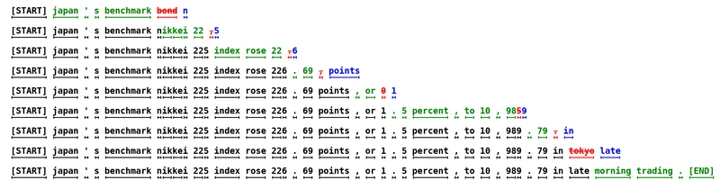
Figure 1 of Fast Inference from Transformers via Speculative Decoding (arXiv:2211.17192), reproduced for editorial coverage.

Section 3: Problem formalisation

Notation table

Symbol	Type	Meaning	First appears
$M_p$	Model	Target (large) model with distribution $p(\cdot \mid \text{prefix})$	Section 3
$M_q$	Model	Draft (small / auxiliary) model with distribution $q(\cdot \mid \text{prefix})$	Section 3
$\gamma$	Integer	Number of speculative tokens drafted per step	Section 3
$\alpha$	$[0, 1]$	Per-token acceptance rate, averaged over the data distribution	Section 3
$\tau$	Real $\geq 1$	Expected accepted tokens per target forward pass	Section 6
$f_i$	Vector $\in \mathbb{R}^d$	Second-to-top hidden-layer feature at position $i$ (EAGLE)	Section 5
$e_i$	Vector $\in \mathbb{R}^d$	Token embedding at position $i$	Section 5
$h_t$	Vector $\in \mathbb{R}^d$	Final hidden state at decode step $t$ (Medusa)	Section 5

Formal problem statement

Autoregressive decoding from an LLM is sequential by construction: generating the $(t+1)$-th token requires a forward pass conditioned on tokens $1$ through $t$. The latency floor is therefore one full forward pass per output token. For a 70B-parameter model running on a single GPU, each forward pass is dominated by memory bandwidth — moving the model’s weights from HBM to compute units — not by arithmetic throughput. From the paper: “the bottleneck of LLM inference is largely memory bandwidth and communication, so faster inference can often be achieved by better utilizing the available compute.” ³

The four papers all solve the same formal problem: produce a decoder that emits tokens drawn from the target distribution $p$, but with strictly fewer than one target-model forward pass per emitted token, on average, on real prompt distributions.

Lossless property — speculative sampling derivation

From the Leviathan paper: ¹ given draft distribution $q(x)$ and target distribution $p(x)$, accept a draft sample $x$ with probability

$\text{accept}(x) = \min\!\left(1,\ \frac{p(x)}{q(x)}\right).$

If rejected, draw a replacement from the residual distribution

$p'(x) = \frac{\max(0,\ p(x) - q(x))}{\sum_{x'} \max(0,\ p(x') - q(x'))}.$

[Reconstructed] The proof that the accepted token is distributed as $p$ is one line: the joint probability that token $x$ is sampled from $q$ AND accepted is $q(x) \cdot \min(1, p(x)/q(x)) = \min(q(x), p(x))$. The probability that a rejection occurs AND the replacement equals $x$ is $\big(1 - \sum_{x'} \min(q(x'), p(x'))\big) \cdot p'(x) = \max(0, p(x) - q(x))$. Adding the two gives exactly $p(x)$. Losslessness is therefore not approximate; it is an algebraic identity.

Assumptions

• The draft model’s distribution $q$ is computable cheaply. From the paper: Leviathan recommends $q$ run at roughly $1/c$ the per-token cost of $p$ where $c$ is somewhere in the range 10-100 depending on the model pair. ¹
• The target model can run a batched forward pass on $\gamma + 1$ prefixes (the $\gamma$ drafted tokens plus the rejection-replacement position) at roughly the same wall-clock cost as a single-token forward pass, because LLM inference is memory-bandwidth-bound. [Analysis] This assumption holds well at batch size 1; it weakens as batch size grows because parallel verification competes with batched user requests for the same HBM bandwidth.
• For Medusa and EAGLE: the target model can be augmented with extra parameters (decoding heads in Medusa, a single decoder layer in EAGLE) without disturbing its output distribution. Medusa-1 keeps the target frozen; EAGLE always keeps the target frozen. ^{2 3}

Why the problem is hard

The acceptance rate $\alpha$ is bounded above by how well $q$ approximates $p$. From the paper: Leviathan’s analysis shows that the expected tokens generated per target forward pass is

$E[\#\text{tokens}] = \frac{1 - \alpha^{\gamma + 1}}{1 - \alpha}.$

For $\alpha = 0.7$ and $\gamma = 4$, this evaluates to roughly $2.85$ tokens per pass. ¹ The whole game is squeezing $\alpha$ closer to 1 without making the draft so expensive that the per-pass time blows up. [Analysis] Medusa, EAGLE, and EAGLE-2 are best read as successive attempts to win on this trade-off curve.

Section 4: Motivation and gap

LLM inference latency has become the binding constraint on user-facing applications: chat completion, code suggestion in IDEs, agent reasoning loops. [External comparison] Throughput-oriented techniques like FlashAttention, paged KV cache (vLLM), and quantisation reduce per-pass cost but do not change the sequential ceiling of one forward pass per token.

Earlier work explored two parallel lines:

• Non-autoregressive decoding — predict all output tokens in parallel from a single forward pass. [External comparison] This sacrifices quality, especially for tasks with high entropy at each position.
• Block-wise parallel decoding (Stern et al. 2018; Sun et al. 2021). [External comparison] Earlier than Leviathan; predicts several tokens at once but without the rejection-sampling guarantee, so output distribution shifts.

The gap Leviathan’s paper claims to fill: exact losslessness at non-trivial speedup, with no architectural change to the target model. ¹ A concurrent paper from DeepMind by Chen et al. (arXiv:2302.01318) derived essentially the same procedure independently under the name “speculative sampling.” ⁵ [External comparison] The community generally credits both papers jointly as the origin of the modern method.

The gap Medusa’s paper claims to fill: avoid the operational burden of having a separate, well-aligned draft model. From the paper: training and serving a smaller draft model that mimics the larger model’s outputs adequately is a meaningful engineering tax. ² Medusa proposes that the heads can be trained from frozen target features in hours, on a single A100.

The gap EAGLE’s paper claims to fill: tokens are inherently uncertain (a model genuinely cannot tell which of two plausible next tokens will be sampled), but the features one layer down are far less uncertain. From the paper: “autoregression at the feature (second-to-top-layer) level is more straightforward than at the token level.” ³ Drafting on features should therefore push $\alpha$ higher than Medusa’s approach.

The gap EAGLE-2’s paper claims to fill: EAGLE’s static draft tree wastes draft budget at low-confidence positions (where most candidate paths will be rejected) and underspends at high-confidence positions (where deeper trees would harvest more accepted tokens). From the paper: a context-dependent dynamic tree should outperform a one-size-fits-all static tree. ⁴

Section 5: Method overview, paper by paper

5A — Leviathan speculative decoding

Pipeline. Given a current prefix, the draft model $M_q$ autoregressively produces $\gamma$ tokens. The target $M_p$ then runs a single batched forward pass on the prefix plus all $\gamma$ drafted positions, producing $\gamma + 1$ next-token distributions. Each drafted token is accepted or rejected via $\min(1, p/q)$; the first rejected position is replaced by a sample from the residual $p'$. Accepted tokens plus the replacement (one or zero of them) are committed; the loop restarts.

[Reconstructed] The maximum tokens committed per outer iteration is $\gamma + 1$ (all $\gamma$ drafts accepted, plus one bonus token sampled directly from $p$ at the position after the last accepted draft, since the target has already computed its distribution there for free).

Why it works mechanically. Modern accelerators (TPU-v4, A100, H100) have peak FLOPS far exceeding what a single sequence’s forward pass uses. Running the target on $\gamma + 1$ prefixes in parallel is barely more expensive than on one, as long as the KV cache and weight reads dominate. The draft model is small enough that its $\gamma$ sequential passes are cheap.

Classification. [New] — the rejection-sampling formulation with the residual distribution was new. The draft-and-verify intuition predates the paper, but the lossless proof did not.

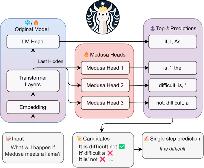
Figure 1 of Medusa: Simple LLM Inference Acceleration Framework with Multiple Decoding Heads (arXiv:2401.10774), reproduced for editorial coverage.

5B — Medusa

Pipeline. Bolt $K$ extra decoding heads onto the target model. Each head $k$ predicts the token at position $t + k + 1$ from the target’s final hidden state $h_t$. All heads run in parallel from the same hidden state, so the draft cost is one target forward pass plus $K$ small MLP evaluations.

From the paper: the heads are MLPs with a SiLU activation and a residual connection. The $k$-th head computes

$p_t^{(k)} = \mathrm{softmax}\!\left(W_2^{(k)} \cdot \big(\mathrm{SiLU}(W_1^{(k)} \cdot h_t) + h_t\big)\right),$

with $W_1^{(k)} \in \mathbb{R}^{d \times d}$ and $W_2^{(k)} \in \mathbb{R}^{d \times V}$. ²

Tree attention. Each head emits its top-$s_k$ candidates, giving up to $\prod_k s_k$ candidate continuations. A tree attention mask lets the target verify all of them in one batched forward pass without cross-contamination — each token attends only to its ancestors in the tree.

Medusa-1 vs Medusa-2. Medusa-1 trains only the heads with the backbone frozen. Medusa-2 jointly fine-tunes the heads and the backbone with a carefully tuned recipe that preserves backbone quality. From the paper: Medusa-1 is lossless; Medusa-2 is near-lossless because the backbone has been updated. ²

Typical acceptance. When sampling at temperature > 0, the standard speculative-sampling rejection rule is statistically valid but rejects too many high-entropy candidates. Medusa replaces it with a typical-acceptance rule that accepts $x_{n+k}$ when

$p_{\text{original}}(x_{n+k} \mid \ldots) > \min\!\big(\varepsilon,\ \delta \cdot \exp(-H(p_{\text{original}}(\cdot \mid \ldots)))\big),$

where $H$ denotes entropy. ² [Analysis] This is a quality-preserving heuristic that strictly drops the lossless guarantee at temperature > 0 — the output distribution may diverge from $p$, though the paper argues empirical quality is preserved on MT-Bench.

Classification. [Adapted] — extends Leviathan’s framework by removing the separate draft model. The tree-attention idea is a meaningful elaboration of Leviathan’s single-chain verification.

5C — EAGLE

Key insight. Token-level sampling is genuinely uncertain (the next token may be one of several near-equiprobable choices). But the feature $f_i$ at the second-to-top transformer layer encodes the model’s “decision” about what is being predicted, and is much less uncertain than the eventual sampled token. From the paper: drafting on features rather than tokens should push $\alpha$ higher. ³

Auto-regressive head. A single transformer decoder layer takes as input a fused sequence: the feature $f_i$ at position $i$ concatenated with the next position’s token embedding $e_{i+1}$. Concatenating $e_{i+1}$ — the token that the target actually committed at position $i+1$ — resolves the feature-level uncertainty that arises from not yet knowing which of several plausible tokens was sampled. ³

Loss. Train the head with a weighted sum of a Smooth-L1 regression loss on predicted vs. ground-truth features and a cross-entropy classification loss on the predicted tokens via the (frozen) LM head:

$\mathcal{L} = \mathcal{L}_{\text{reg}} + w_{\text{cls}} \cdot \mathcal{L}_{\text{cls}}, \quad w_{\text{cls}} = 0.1.$

From the paper: only the new transformer decoder layer is trained; the target model stays frozen. ³

Tree drafting. Like Medusa, EAGLE drafts a tree of candidate continuations. The tree is static — same shape every drafting step — and the head runs autoregressively along the tree for $\gamma$ steps.

Classification. [New] — the move from token-level to feature-level drafting is a genuinely novel contribution; the rest of the pipeline (rejection sampling, tree attention) is adopted from Leviathan and Medusa.

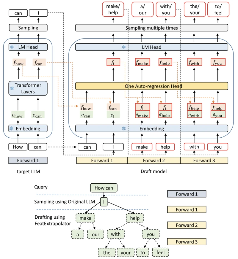
Figure 6 of EAGLE: Speculative Sampling Requires Rethinking Feature Uncertainty (arXiv:2401.15077), reproduced for editorial coverage.

5D — EAGLE-2

Key insight. EAGLE’s static tree gives every drafting step the same shape regardless of context. But the draft model’s own confidence at each node is a strong predictor of whether the target will accept the token. From the paper: confidence < 0.05 corresponds to acceptance rate of approximately 0.04, while confidence > 0.95 corresponds to acceptance rate of approximately 0.98. ⁴

Algorithm. Two stages per drafting step:

1. Expand. Compute, for every leaf of the current draft tree, a global acceptance value $V_i$ defined as the product of the draft model’s confidence scores along the path from root to node $i$. Pick the top-$k$ leaves by $V_i$ and run the EAGLE head one more step from each. From the paper: $V_i = \prod \text{confidence scores along path}$. ⁴
2. Rerank. Across the entire (now-larger) tree, rerank all draft tokens by $V_i$ and select the top $m$ tokens to forward to the target for verification. Ties broken toward shallower nodes to keep the tree connected. ⁴

What changes vs EAGLE. The draft model is identical to EAGLE — same weights, same architecture, same training recipe. Only the tree-construction logic at inference time changes. From the paper: “EAGLE-2 does not modify the structure of the draft model.” ⁴

Classification. [Adapted] — a serving-time refinement of EAGLE, not a new draft architecture.

Section 6: Mathematical contributions

MATH ENTRY [1]: Expected tokens per target forward pass

• Source: Leviathan, Section 3.2 / Eq. (1)-(2). ¹

• What it is: A closed-form formula for how many tokens the speculative-decoding loop commits per target forward pass, given the draft model’s acceptance rate $\alpha$ and the number of drafted tokens $\gamma$.

• Formal definition:

  $E[\#\text{tokens}] = \frac{1 - \alpha^{\gamma + 1}}{1 - \alpha}.$

• Each term explained + dimensional analysis:

  • $\alpha \in [0, 1]$ is the per-token acceptance rate (dimensionless probability).
  • $\gamma \in \mathbb{Z}_{\geq 1}$ is the number of draft tokens per step (positive integer).
  • $E[\#\text{tokens}]$ is dimensionless and lies in the interval $[1,\ \gamma + 1]$ (sanity check: when $\alpha = 0$, the formula gives 1 — only the bonus token sampled from $p$; when $\alpha \to 1$, the formula approaches $\gamma + 1$).

• Worked numerical example:

  • Take $\alpha = 0.7$, $\gamma = 4$. Numerator: $1 - 0.7^5 = 1 - 0.16807 = 0.83193$. Denominator: $1 - 0.7 = 0.3$. Ratio: $0.83193 / 0.3 = 2.77$ tokens per target pass.
  • Now $\alpha = 0.9$, $\gamma = 4$. Numerator: $1 - 0.9^5 = 1 - 0.59049 = 0.40951$. Denominator: $0.1$. Ratio: $4.10$ tokens per target pass.
  • And $\alpha = 0.5$, $\gamma = 4$. Numerator: $1 - 0.5^5 = 0.96875$. Denominator: $0.5$. Ratio: $1.94$.
  • [Analysis] The function is highly nonlinear in $\alpha$ near 1. Pushing $\alpha$ from 0.7 to 0.9 at $\gamma=4$ buys 1.5x more tokens per pass; pushing it from 0.5 to 0.7 buys only 0.8x more.

• Role: This is the governing equation of the lineage. Every subsequent paper (Medusa, EAGLE, EAGLE-2) is engineered to push $\alpha$ higher or to make $\gamma$ vary cleverly with context.

• Edge cases: Formula undefined at $\alpha = 1$ (limit is $\gamma + 1$); valid for any $\alpha \in [0, 1)$.

• Novelty: [New] — Leviathan’s contribution.

• Why it matters: Quantifies the speedup ceiling for a given draft model in closed form. If a designer measures $\alpha$ on their data distribution, they can predict $E[\#\text{tokens}]$ before benchmarking.

MATH ENTRY [2]: Rejection-sampling acceptance rule

• Source: Leviathan, Section 3.1; same rule appears in Chen et al. (2302.01318), Medusa (when not using typical acceptance), EAGLE, EAGLE-2. ^{1 5}
• What it is: The decision rule that determines whether a draft-proposed token is committed to the output or replaced.
• Formal definition: Given draft distribution $q$ and target distribution $p$ at the same position, draft sample $x \sim q$, accept with probability $\min(1,\ p(x)/q(x))$. If rejected, sample replacement from residual $p'(x) = \mathrm{norm}\!\big(\max(0, p(x) - q(x))\big)$.
• Each term + dimensional analysis:
  • $p(x), q(x) \in [0, 1]$ are scalar probabilities, summing to 1 over vocabulary $V$.
  • $p(x)/q(x)$ is the importance ratio; undefined if $q(x) = 0$ (handled by definition: rejection if $q(x) = 0$ and $p(x) > 0$, which the draft never samples).
  • $p'(x)$ is a normalised probability distribution over the same vocabulary $V$.
• Worked numerical example:
  • Vocabulary $V = \{a, b, c\}$. Target $p = [0.6, 0.3, 0.1]$. Draft $q = [0.4, 0.4, 0.2]$.
  • Draft samples $x = a$ with probability 0.4. Acceptance probability $= \min(1, 0.6/0.4) = \min(1, 1.5) = 1$. Always accept.
  • Draft samples $x = b$ with probability 0.4. Acceptance probability $= \min(1, 0.3/0.4) = 0.75$. Accept 75%, reject 25%.
  • Draft samples $x = c$ with probability 0.2. Acceptance probability $= \min(1, 0.1/0.2) = 0.5$.
  • Residual at rejection: $\max(0, p - q) = [\max(0, 0.2), \max(0, -0.1), \max(0, -0.1)] = [0.2, 0, 0]$. Normalised: $p' = [1, 0, 0]$. So rejection always replaces with token $a$.
  • Verify marginal: probability of emitting $a$ = (drew $a$ and accepted) + (drew $b$ and rejected, replaced with $a$) + (drew $c$ and rejected, replaced with $a$) $= 0.4 \cdot 1 + 0.4 \cdot 0.25 \cdot 1 + 0.2 \cdot 0.5 \cdot 1 = 0.4 + 0.1 + 0.1 = 0.6$. Exactly $p(a)$. Losslessness holds.
• Role: The single guarantee that makes the entire lineage lossless rather than quality-degrading.
• Edge cases: When draft and target agree perfectly, $\alpha = 1$ for every token and replacements never fire. When they disagree completely, residual is identical to $p$ and the draft never helps.
• Novelty: [New] — Leviathan and Chen et al. arrived independently.
• Why it matters: Distinguishes speculative decoding from non-autoregressive decoding or block parallel decoding, both of which sacrifice exactness for speed.

MATH ENTRY [3]: Medusa decoding head

• Source: Medusa, Section 3.1. ²

• What it is: The MLP-with-residual that maps the target’s final hidden state to a token distribution at a future position.

• Formal definition:

  $p_t^{(k)} = \mathrm{softmax}\!\left(W_2^{(k)} \cdot \big(\mathrm{SiLU}(W_1^{(k)} \cdot h_t) + h_t\big)\right).$

• Each term + dimensional analysis:

  • $h_t \in \mathbb{R}^d$ — target’s final hidden state at position $t$. For LLaMA-7B, $d = 4096$.
  • $W_1^{(k)} \in \mathbb{R}^{d \times d}$ — first projection. Dim: $d \times d$ matrix.
  • $\mathrm{SiLU}(x) = x \cdot \sigma(x)$, applied elementwise. Returns $\mathbb{R}^d$.
  • Residual $\mathrm{SiLU}(W_1^{(k)} h_t) + h_t \in \mathbb{R}^d$.
  • $W_2^{(k)} \in \mathbb{R}^{d \times V}$ — output projection. Dim: $d \times V$. For LLaMA-7B with $V = 32{,}000$, this is the dominant parameter cost.
  • $p_t^{(k)} \in [0, 1]^V$ — token distribution at position $t + k + 1$.

• Worked numerical example: Take $d = 8$, $V = 4$. Suppose $h_t = [1, 0, -1, 2, 0, 1, -2, 1]$. $W_1^{(k)}$ is the $8 \times 8$ identity matrix; then $W_1^{(k)} h_t = h_t$. $\mathrm{SiLU}(h_t) \approx [0.73, 0, -0.27, 1.76, 0, 0.73, -0.24, 0.73]$. Residual: $h_t + \mathrm{SiLU}(h_t) \approx [1.73, 0, -1.27, 3.76, 0, 1.73, -2.24, 1.73]$. $W_2^{(k)}$ has shape $8 \times 4$; suppose its first row picks coordinate 4 strongly. The pre-softmax logit vector has length 4; softmax then yields a probability distribution over the 4-token vocabulary.

• Role: Predicts token at position $t + k + 1$ in parallel with the target’s normal next-token head. $K$ heads in parallel give a $K$-deep draft from one forward pass.

• Edge cases: Head accuracy degrades with $k$ — the further ahead a head predicts, the worse it does. From the paper: top-1 accuracy of the 1st head is around 60% on Vicuna-7B vs around 30% for the 5th head. ²

• Novelty: [Adapted] from block parallel decoding (Stern 2018); the residual MLP design and joint use with tree attention are Medusa’s elaboration.

• Why it matters: Removes the separate draft-model dependency entirely. The “draft” is now just additional parameters trained on top of the target.

MATH ENTRY [4]: EAGLE feature-level autoregression loss

• Source: EAGLE, Section 3. ³

• What it is: The training objective for EAGLE’s single decoder layer, which predicts the next-position feature given the current feature and the next token embedding.

• Formal definition:

  $\mathcal{L} = \mathcal{L}_{\text{reg}}\big(\hat{f}_{i+1},\ f_{i+1}\big) + w_{\text{cls}} \cdot \mathcal{L}_{\text{cls}}\big(\mathrm{LMHead}(\hat{f}_{i+1}),\ y_{i+1}\big), \quad w_{\text{cls}} = 0.1.$

• Each term + dimensional analysis:

  • $f_{i+1} \in \mathbb{R}^d$ — ground-truth second-to-top feature at position $i+1$ (collected by running the target on training data).
  • $\hat{f}_{i+1} \in \mathbb{R}^d$ — predicted feature from EAGLE’s decoder layer given input $[f_i;\ e_{i+1}]$ (concatenation along feature dim).
  • $\mathcal{L}_{\text{reg}}$ — Smooth-L1 (Huber) loss, scalar.
  • $\mathcal{L}_{\text{cls}}$ — cross-entropy between target’s LM-head output on $\hat{f}_{i+1}$ and the ground-truth next token $y_{i+1}$, scalar.
  • $w_{\text{cls}} = 0.1$ — fixed scalar weight.

• Worked numerical example: Suppose $d = 4$, $\hat{f}_{i+1} = [1.0, 0.5, -0.2, 0.0]$, $f_{i+1} = [1.1, 0.4, -0.3, 0.1]$. Per-dim absolute differences: $[0.1, 0.1, 0.1, 0.1]$. All below Smooth-L1 threshold 1.0, so Smooth-L1 returns $\sum 0.5 \cdot 0.1^2 = 4 \cdot 0.005 = 0.02$. For the cross-entropy term: passing $\hat{f}_{i+1}$ through the frozen LM head produces a vocabulary distribution; if the ground-truth token’s predicted probability is 0.4, cross-entropy is $-\log 0.4 \approx 0.916$. Total loss: $0.02 + 0.1 \cdot 0.916 = 0.112$.

• Role: Trains the EAGLE head to predict the next feature and the next token consistently, leveraging the (frozen) LM head as a shared decoder.

• Edge cases: If the LM head is fine-tuned post-EAGLE-training, EAGLE’s predictions drift and need retraining.

• Novelty: [New] — joint regression-plus-classification on second-to-top features is the paper’s central training contribution.

• Why it matters: Lets EAGLE’s tiny draft model (one decoder layer) match a much larger draft model’s accuracy at a fraction of the parameter cost.

MATH ENTRY [5]: EAGLE-2 global acceptance value

• Source: EAGLE-2, Section 3. ⁴

• What it is: A scalar score per draft-tree node estimating the marginal probability that the target will accept the token at that node and all its ancestors.

• Formal definition: For node $i$ at depth $D_i$ along path $r \to n_1 \to n_2 \to \cdots \to n_{D_i} = i$ from root $r$:

  $V_i = \prod_{j=1}^{D_i} \mathrm{conf}(n_j),$

  where $\mathrm{conf}(n_j) \in [0, 1]$ is the draft model’s output probability for node $n_j$ given its prefix.

• Each term + dimensional analysis:

  • $\mathrm{conf}(n_j)$ — softmax output of the draft model at the position where $n_j$ was generated. Dimensionless probability.
  • $V_i$ — product of dimensionless probabilities, itself a dimensionless probability in $[0, 1]$.
  • $D_i$ — node depth, positive integer.

• Worked numerical example: Suppose a draft tree with root, two children with confidences 0.9 and 0.4, and the 0.9 child has its own child with confidence 0.8. The deeper grandchild’s $V = 0.9 \cdot 0.8 = 0.72$. The shallower sibling’s $V = 0.4$. Even though the grandchild is deeper, its global value is higher — so EAGLE-2 expands toward it first.

• Role: Lets the algorithm spend its draft budget on tree paths likely to be accepted, rather than on a fixed shape that overspends on shallow low-confidence regions.

• Edge cases: As tree depth grows, $V_i$ shrinks geometrically; the algorithm naturally stops expanding deep low-confidence chains.

• Novelty: [New] — EAGLE-2’s central scoring innovation. The draft model is unchanged from EAGLE.

• Why it matters: Buys an additional roughly 20-40% speedup on top of EAGLE-1 without retraining anything.

Section 7: Algorithmic contributions

ALGORITHM ENTRY [1]: SpeculativeDecodingStep (Leviathan)

• Source: Leviathan, Algorithm 1. ¹
• Purpose: One outer iteration of speculative decoding, committing between 1 and $\gamma + 1$ tokens.

Inputs: prefix x_{<t}, target M_p, draft M_q, gamma
Outputs: extended prefix x_{<t'} where t' in [t+1, t+gamma+1]

1. Run M_q autoregressively to produce draft tokens d_1, d_2, ..., d_gamma
   and corresponding draft distributions q_1, ..., q_gamma.
2. Run M_p ONCE on the prefix plus the gamma drafted positions in parallel,
   producing target distributions p_1, p_2, ..., p_gamma, p_{gamma+1}.
3. For k = 1 ... gamma:
     r ~ Uniform(0, 1)
     if r <= min(1, p_k(d_k) / q_k(d_k)):
       commit d_k; continue
     else:
       sample replacement r_k ~ p'_k = norm(max(0, p_k - q_k))
       commit r_k; STOP the loop (rest of draft discarded)
4. If all gamma drafts accepted:
     sample bonus token b ~ p_{gamma+1}; commit b.
5. Return extended prefix.

• Hand-traced example. Take vocabulary $\{a, b, c\}$, $\gamma = 2$, $\alpha$ around 0.7 for illustration. Start prefix [start].

  1. Draft runs: produces $d_1 = a$ with $q_1(a) = 0.5$, $d_2 = b$ with $q_2(b) = 0.6$.
  2. Target runs in parallel on prefix and prefix+$a$: produces $p_1(a) = 0.7$, $p_2(b) = 0.4$, $p_3 = [0.5, 0.3, 0.2]$.
  3. $k=1$: ratio $= 0.7/0.5 = 1.4 \geq 1$. Accept $a$.
  4. $k=2$: ratio $= 0.4/0.6 \approx 0.67$. Sample $r$ uniformly. If $r \leq 0.67$, accept $b$; if $r > 0.67$, reject. Suppose $r = 0.8$: reject. Residual: $\max(0, p_2 - q_2)$ for each token. If $p_2 = [0.3, 0.4, 0.3]$ and $q_2 = [0.2, 0.6, 0.2]$, residual = $[0.1, 0, 0.1]$, normalised to $[0.5, 0, 0.5]$. Sample replacement, say $a$. Commit $a$. Stop.
  5. Final committed sequence: [start] a a. The bonus token (step 4) does not fire because the loop stopped at $k=2$.

• Complexity.

  • Time: 1 target forward pass + $\gamma$ draft forward passes per outer iteration. Bottleneck: the target pass (memory-bandwidth-bound on large models).
  • Space: $O(\gamma)$ extra KV cache slots per outer iteration.

• Hyperparameters. $\gamma$ (number of drafts). Higher $\gamma$ gives more parallelism but degrades when $\alpha$ is low (early rejection wastes the deeper drafts). Leviathan reports $\gamma \in \{3, 5, 7\}$ as typical sweet spots. ¹

• Failure modes. When $\alpha$ is very low (poor draft alignment), expected tokens per pass $\to 1$ and the overhead of running the draft becomes pure waste.

• Novelty: [New].

• Transferability: [Analysis] Applies to any pair of (target, draft) models that share a vocabulary and tokeniser. Vocabulary mismatch is the most common operational blocker.

ALGORITHM ENTRY [2]: Medusa parallel-head drafting with tree attention

• Source: Medusa, Section 3.2. ²
• Purpose: Replace the separate draft model with $K$ parallel heads that all consume the target’s final hidden state, generating a tree of candidate continuations verified in one target forward pass.

Inputs: prefix x_{<t}, target M_p with K medusa heads, top-s_k per head
Outputs: extended prefix

1. Run M_p once on prefix, obtain hidden state h_t and head outputs.
2. For each head k = 1 ... K:
     Take top-s_k tokens from head k's distribution -> candidate set C_k.
3. Form candidate tree: Cartesian product over k of C_k.
   Apply tree attention mask so each path is verified independently.
4. Run M_p once with tree-attention input over all tree paths in parallel.
5. For each path, apply typical-acceptance rule along the path.
   Pick the longest accepted prefix across paths -> commit.

• Hand-traced example. Take $K = 3$ heads, top-2 each. Prefix is “The cat”.
  1. Heads emit head-1 = {sat, jumped}, head-2 = {on, over}, head-3 = {the, a}.
  2. Tree has $2 \times 2 \times 2 = 8$ candidate continuations: sat on the, sat on a, sat over the, …, jumped over a.
  3. Tree-attention mask: token on in path sat on the attends to The cat sat but not to jumped. Token the attends to The cat sat on.
  4. One batched forward pass through the target verifies all 8 paths in parallel.
  5. Typical-acceptance on path sat on the: accept if $p_{\text{target}}(\text{sat} \mid \text{The cat}) > \min(\varepsilon, \delta e^{-H})$, then accept on given The cat sat, etc. Pick the longest accepted prefix.
• Complexity. 1 target forward pass per outer iteration (vs $\gamma + 1$ in Leviathan, but with $\prod_k s_k$ tree branches in the verification pass). Memory cost in KV cache grows with tree size.
• Hyperparameters. $K = 5$ heads in Medusa’s main experiments. Top-$s_k$ values tuned per head; from the paper, head-1 might use $s_1 = 10$ while head-5 uses $s_5 = 1$. ²
• Failure modes. Head accuracy degrades steeply with $k$. Joint top-$s$ tree blows up combinatorially; the paper uses a hand-tuned sparse tree shape.
• Novelty: [Adapted] from block-wise parallel decoding plus Leviathan’s verification rule.
• Transferability: [Analysis] Generic across decoder-only transformer architectures. Requires fine-tuning the heads on the target’s own outputs.

ALGORITHM ENTRY [3]: EAGLE-2 dynamic draft-tree expansion

• Source: EAGLE-2, Section 3. ⁴
• Purpose: Build, per drafting step, a context-dependent draft tree whose shape reflects per-token confidence.

Inputs: prefix x_{<t}, EAGLE draft head H, top-k expansion budget, top-m forward budget
Outputs: draft tree to verify

1. Run target M_p once on prefix; obtain feature f_t.
2. Initialize tree with root holding f_t.
3. EXPANSION (repeated for several layers):
     For every leaf of current tree, run H once to obtain child distributions.
     For every candidate (parent, child token c) pair:
       conf(c) := draft probability of c given parent's hidden state.
       V_{new leaf} := V_{parent} * conf(c).
     Pick top-k new leaves by V; add them as children. Discard the rest.
4. RERANK across the full grown tree:
     Pick top-m nodes overall by V (tie-break toward shallower depth).
5. Construct tree-attention mask over selected m nodes.
6. Run M_p once over the tree; verify via speculative-sampling rule.

• Hand-traced example. Take expansion budget $k = 3$, forward budget $m = 5$. Root feature corresponds to prefix “Hello”.
  1. Draft head proposes children: world (conf 0.7), there (conf 0.2), everyone (conf 0.1). Their $V$: 0.7, 0.2, 0.1.
  2. Pick top-3 (all three, in this case).
  3. From world ($V = 0.7$), draft proposes: , (conf 0.6), ! (conf 0.3). New $V$: 0.42, 0.21.
  4. From there ($V = 0.2$), draft proposes: , (conf 0.8), ! (conf 0.1). New $V$: 0.16, 0.02.
  5. From everyone ($V = 0.1$), draft proposes: , (conf 0.7). New $V$: 0.07.
  6. Now rerank across the entire tree (nodes plus their grown children) by $V$: world (0.7), world, (0.42), there (0.2), world! (0.21), there, (0.16). Pick top-5.
  7. Target verifies all 5 in one tree-attention forward pass.
• Complexity. One extra forward pass through the draft head per expansion layer, plus one target forward pass. Total target passes per outer iteration is unchanged from EAGLE.
• Hyperparameters. Expansion budget per layer, total forward budget $m$, number of expansion layers. From the paper: typical values are layered expansion up to 6 layers deep with budget around 60. ⁴
• Failure modes. When the draft model’s confidence is poorly calibrated (a known LLM pathology), the global acceptance values mis-rank candidates and the dynamic tree loses to a well-tuned static tree.
• Novelty: [New] — the global-acceptance scoring and expand-then-rerank procedure.
• Transferability: [Analysis] Drop-in replacement for EAGLE’s static tree at inference time. Requires no retraining.

Section 8: Specialised design contributions

8A — LLM / prompt design

Not applicable to this paper cluster. Speculative decoding is an inference-system technique, not a prompting technique.

8B — Architecture-specific details

• Medusa heads are MLPs with a residual SiLU activation; each head has roughly $d \times d + d \times V$ parameters. For LLaMA-7B ($d = 4096$, $V = 32{,}000$), one head adds approximately 150M parameters; with $K = 5$ heads, roughly 750M extra parameters, which is non-trivial relative to the 7B target. ²
• EAGLE head is a single transformer decoder layer at the target’s hidden dimension. For LLaMA-7B, this adds approximately 0.24B parameters — meaningfully smaller than Medusa’s stack of 5 MLPs. ³
• Tree attention in both Medusa and EAGLE is implemented as a sparse causal mask. Each position attends only to its ancestors in the tree, not to siblings.

8C — Training specifics

• Medusa-1 training. From the paper: 5 heads with 1 layer each, trained on the ShareGPT dataset (around 60k samples) for one epoch, taking approximately 5 hours on a single NVIDIA A100 PCIE GPU. Backbone frozen. ²
• Medusa-2 training. Joint fine-tuning of heads + backbone using a two-stage recipe (warm up heads first, then differential learning rates). From the paper: preserves backbone quality on MT-Bench. ²
• EAGLE training. From the paper: train the single decoder-layer head on data generated by the target itself (the target’s own (feature, token) sequences). Loss as in MATH ENTRY [4]. Target frozen throughout. ³
• EAGLE-2 training. Same training as EAGLE; only inference changes. ⁴

8D — Inference / deployment specifics

• All four methods require the target model’s KV cache to be addressable for tree-attention verification.
• Medusa and EAGLE both modify the verification forward pass to consume tree-shaped inputs; this requires a custom CUDA kernel or a compatible attention implementation (e.g., FlashAttention with custom mask).
• EAGLE-2 reuses EAGLE’s inference kernels with only the tree-construction loop modified.
• Production frameworks that ship support for one or more of these methods include vLLM, TensorRT-LLM, and SGLang. [External comparison] vLLM in particular has shipped Medusa support since 2024 and EAGLE support since mid-2024.

Section 9: Experiments and results

Datasets and benchmarks

Paper	Primary benchmarks	Task type
Leviathan	WMT EnDe (translation), CNN/Daily Mail (summarisation)	Encoder-decoder T5
Medusa	MT-Bench	Chat / instruction following
EAGLE	MT-Bench, HumanEval, GSM8K, Alpaca	Chat + code + math
EAGLE-2	MT-Bench, HumanEval, GSM8K, Alpaca, Spec-Bench	As EAGLE plus benchmarking suite

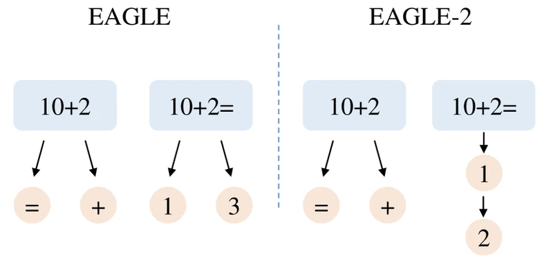
Figure 4 of EAGLE-2: Faster Inference of Language Models with Dynamic Draft Trees (arXiv:2406.16858), reproduced for editorial coverage.

9A — Leviathan headline numbers

From the paper, Table 2: ¹

Target	Draft	Dataset	Temperature	Speedup
T5-XXL (11B)	T5-small (77M)	WMT EnDe	T=0	3.4x
T5-XXL	T5-small	WMT EnDe	T=1	2.6x
T5-XXL	T5-base (250M)	WMT EnDe	T=0	2.8x
T5-XXL	T5-large (800M)	WMT EnDe	T=0	1.7x
T5-XXL	T5-small	CCN/DM	T=0	3.1x
T5-XXL	T5-base	CCN/DM	T=0	3.0x
T5-XXL	T5-large	CCN/DM	T=0	2.2x

Acceptance rates $\alpha$ ranged from 0.53 to 0.82 across the configurations. ¹

Hardware: TPU-v4 with batch size 1. ¹

[Analysis] A non-monotone pattern: the smallest draft (T5-small, 1/143 the target size) gives the highest speedup on EnDe, while the largest draft (T5-large, 1/14 the target size) gives the lowest. This is the central trade-off: a bigger draft pushes $\alpha$ up but pushes the per-draft-token cost up faster.

9B — Medusa headline numbers

From the paper, Tables 1-3: ²

Target	Method	MT-Bench speedup	MT-Bench quality
Vicuna-7B	Medusa-1	2.18x	preserved
Vicuna-7B	Medusa-2	2.83x	6.18
Vicuna-13B	Medusa-1	2.33x	preserved
Vicuna-13B	Medusa-2	2.83x	6.43
Vicuna-33B	Medusa-2 (self-distilled)	2.3x	7.18
Zephyr-7B	Medusa-2	3.14x (acceleration rate)*	7.25

* Medusa reports “acceleration rate” and overhead separately; the wall-clock speedup on Zephyr-7B is approximately 2.66x after the 1.18x overhead.

Hardware: NVIDIA A100 PCIE GPU. ²

9C — EAGLE headline numbers

From the paper, Tables 4-6, temperature = 0: ³

Target	Speedup (low end)	Speedup (high end)	$\tau$ tokens / pass
Vicuna 7B	2.79x	3.33x	3.86 - 4.29
Vicuna 13B	3.03x	3.58x	3.95 - 4.39
Vicuna 33B	2.97x	3.67x	3.61 - 4.28
LLaMA2-Chat 7B	2.78x	3.17x	3.71 - 4.24
LLaMA2-Chat 13B	3.01x	3.76x	3.83 - 4.52
LLaMA2-Chat 70B	2.97x	3.52x	3.77 - 4.42
Mixtral 8x7B Instruct	1.50x	1.50x	3.25

EAGLE + gpt-fast on LLaMA2-Chat 7B running on RTX 3090: 160.4 tokens/sec. ³

Hardware: A100 40G and RTX 3090. ³

Versus Medusa-1 and Lookahead: “1.7x-2.1x and 1.5x-1.6x speedups, respectively.” ³

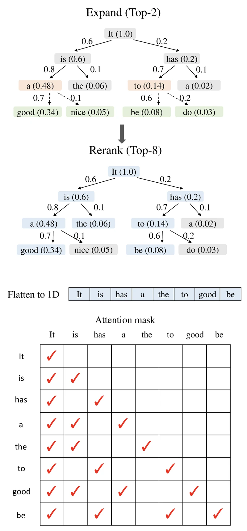
Figure 7 of EAGLE-2: Faster Inference of Language Models with Dynamic Draft Trees (arXiv:2406.16858), reproduced for editorial coverage.

9D — EAGLE-2 headline numbers

From the paper: ⁴

Target	Dataset	EAGLE-2 speedup	EAGLE-1 speedup	Relative gain
Vicuna 13B	MT-Bench	4.26x	3.07x	+39%
Vicuna 13B	HumanEval	4.96x	3.58x	+39%
LLaMA2-Chat 13B	MT-Bench	4.21x	3.03x	+39%
LLaMA2-Chat 13B	GSM8K	4.31x	3.20x	+35%
LLaMA3-Instruct 70B	MT-Bench	3.51x	3.01x	+17%

Average accepted tokens per drafting step: 4 - 5.5 tokens, “roughly twice that of standard speculative sampling and Medusa.” ⁴

[Analysis] The gain over EAGLE narrows on LLaMA3-Instruct 70B (+17%) compared with mid-size models (+35-39%). Either the dynamic-tree budget is calibrated for mid-size models, or larger models’ per-token confidence is less well calibrated, eroding the global-acceptance ranking.

Ablations and stress tests

• Leviathan ablates $\gamma$ from 1 to 7, showing the closed-form prediction matches measured speedups within a few percent. ¹
• Medusa ablates the number of heads (1 - 5), confirming diminishing returns past 4. ²
• EAGLE ablates the LM-head loss weight $w_{\text{cls}}$ at 0.0 / 0.1 / 1.0, finding 0.1 optimal. ³
• EAGLE-2 ablates the expansion budget and total forward budget separately; the optimal frontier sits at expansion 60-80, forward budget around 50-60. ⁴

Independent benchmark cross-checks

Spec-Bench (Xia et al., ACL 2024) ⁹ provides a third-party benchmarking suite for speculative-decoding methods. EAGLE and EAGLE-2 perform near the top of the Spec-Bench leaderboards on most settings. [Reviewer Perspective] The SOTA-claim caveat for the EAGLE-2 paper is that it benchmarks against EAGLE-1 and Medusa under one set of tree budgets; a head-to-head on identical tree budgets and identical hardware was added in the Spec-Bench paper and is the most reliable independent reproducibility check available as of 2026-05.

Evidence audit

• Strongly supported claims. All speedup numbers are reported with measured $\tau$ (tokens per pass) and acceptance rate, allowing the reader to cross-check against the closed-form formula. The lossless property is supported by algebraic proof (Leviathan) plus empirical quality preservation on MT-Bench.
• Partially supported claims. Medusa-2’s “near-lossless” claim — the paper compares MT-Bench scores pre- and post-Medusa-2 training but does not report a distributional test, so claims of equivalence are based on a single coarse benchmark.
• Claims relying on narrow evidence. EAGLE-2’s “20-40%” headline is an average over benchmarks but masks the 17% on LLaMA3-Instruct 70B and the 39% on Vicuna 13B — the dispersion matters for serving teams choosing where to deploy.

Section 10: Technical novelty summary

Component	Type	Novelty level	Justification	Source
Rejection-sampling acceptance rule	Algorithm	Fully novel	Proved exact distribution preservation for the first time	Leviathan §3, Chen et al. concurrent
$E[\#\text{tokens}]$ closed form	Theory	Fully novel	Allows speedup prediction from $\alpha, \gamma$ alone	Leviathan §3.2
Multi-head parallel decoding	Architecture	Combination novel	Block-parallel decoding existed pre-Medusa; combining with tree attention + frozen-backbone training is new	Medusa §3
Tree attention	Algorithm	Incrementally novel	Sparse-mask attention has been used before; using it for parallel verification of multiple candidate continuations is new	Medusa, EAGLE
Feature-level autoregression	Architecture	Fully novel	The shift from token-level to feature-level drafting is the key contribution of EAGLE	EAGLE §3
Feature + next-token input fusion	Architecture	Fully novel	Solving feature uncertainty by feeding next-position token embedding is EAGLE’s specific contribution	EAGLE §3.2
Global acceptance value scoring	Algorithm	Fully novel	Per-node confidence-product scoring for tree shaping is EAGLE-2’s specific contribution	EAGLE-2 §3
Dynamic expand-then-rerank	Algorithm	Fully novel	Two-stage tree growth with global reranking	EAGLE-2 §3

Most novel contribution. EAGLE’s move to second-to-top-feature drafting. [Analysis] It is the only one of the four contributions that exploits a structural insight about the target model itself (its features are less uncertain than its tokens) rather than a serving-system optimisation.

Not claimed novel. Rejection sampling itself (textbook MCMC technique adopted for the lossless guarantee); SiLU activations and decoder-layer building blocks (LLaMA-family standard); MT-Bench, HumanEval, GSM8K, Alpaca benchmarks (community-standard).

Section 11: Situating the work

Prior work

Block-parallel decoding (Stern et al. 2018) and shallow-aggressive decoding (Sun et al. 2021) both attempted to predict multiple future tokens in parallel from a single forward pass, but neither offered a distribution-preserving guarantee — they were quality-degrading techniques the community avoided in production.

What changes

Speculative decoding turned parallel multi-token prediction from a “lossy speedup” into a “lossless speedup,” which is the precondition for serving teams to adopt it at all. Models like LLaMA, GPT-4, and Claude are widely understood to use some form of speculative decoding in production serving — exactly which variant is rarely disclosed publicly.

Two contemporaneous related papers

1. Chen et al. — Accelerating Large Language Model Decoding with Speculative Sampling (arXiv:2302.01318). ⁵ DeepMind’s independent derivation, published two months after Leviathan’s preprint. Same rejection-sampling formula, similar speedup numbers on Chinchilla 70B. [External comparison] The community generally cites Leviathan and Chen et al. jointly.
2. Spec-Bench — Xia et al., ACL 2024. ⁹ An independent benchmarking suite comparing Medusa, EAGLE, EAGLE-2, Lookahead, REST, SpS, and others on a common evaluation harness. The Spec-Bench leaderboard is the closest the community has to an external referee for the four papers’ speedup claims.

[Reviewer Perspective] strongest skeptical objection

The reported speedups are at batch size 1 on a single GPU. [Reviewer Perspective] In production serving — where batch sizes routinely exceed 32 and continuous-batching schedulers (vLLM-style) keep GPUs near saturation — the assumption that the target forward pass on $\gamma + 1$ prefixes is “free” no longer holds. Tree attention with $K = 5$ heads and top-10 each can generate hundreds of speculative positions per request; at batch 64 this is tens of thousands of speculative positions competing for HBM bandwidth that other requests need. EAGLE-2’s dynamic tree partially addresses this by allocating budget per-request, but no paper in the lineage reports speedups on saturated serving workloads.

[Reviewer Perspective] strongest author-side rebuttal

Even at high batch sizes, latency on the first token of each request and on long generations to a single user (agentic loops, large-context Q&A) remains dominated by the per-pass cost. Speculative decoding still wins on those tail latencies even when steady-state throughput gains shrink. [Analysis] The papers’ framing of “speedup” as wall-clock latency at batch 1 is therefore the right metric for the user-perceived experience even if not for cluster throughput.

What remains unsolved

• Speculative decoding’s behaviour under structured outputs (JSON, function calls) where the draft is reasonably accurate but the target imposes a hard grammar constraint at every position. The papers do not report on grammar-constrained decoding.
• Cross-vocabulary settings: when the draft and target have different tokenisers (e.g., a smaller open-weight model drafting for a larger proprietary model with different tokenisation). The papers all assume tokeniser equality.
• Behaviour under speculative thinking steps (chain-of-thought-style generation), where token distributions become long and high-entropy.

Three future directions

1. Draft-tree shaping conditioned on the prompt’s task class. EAGLE-2 shapes by per-token confidence but does not exploit the prior that “this is a code-completion prompt” or “this is GSM8K-style math.” [Analysis] Promising direction surfaced by the EAGLE-2 paper itself.
2. Quantised draft models. Drafts could plausibly run at INT4 or INT2 with minimal $\alpha$ degradation, freeing compute. [Reviewer Perspective] No paper in this lineage explores this.
3. Speculative decoding for agentic workloads. The cost-of-error in an agent is much higher than in chat (a wrong tool call burns money and time). Speculative decoding’s lossless guarantee should be re-examined under tool-augmented decoding, where the next “token” may not be from the model’s vocabulary at all. [Analysis] An open research direction the four papers do not address.

Section 12: Critical analysis

Strengths

• Lossless guarantee with closed-form proof — the rejection-sampling derivation is short, complete, and the foundation of community trust in the method.
• Hardware-grounded. The four papers’ framing of “memory-bandwidth-bound, not compute-bound” is correct and well-substantiated; the technique gets faster on hardware where the gap between FLOPS and HBM bandwidth widens.
• Reproducibility. Both Medusa and EAGLE released code and pretrained draft-model weights under permissive licences. ^{6 7}

Author-stated weaknesses

• Leviathan: works only when an aligned draft model exists; for novel target models, a draft must be trained or selected.
• Medusa: the heads add 5-10% memory overhead at 5 heads on LLaMA-7B; Medusa-2’s joint fine-tuning may cost backbone quality if the recipe is mistuned.
• EAGLE: requires (feature, token) training data from the target’s outputs; if the target is closed-weight, this data has to be collected via API.
• EAGLE-2: per-prompt tree-shaping logic is more CPU-bound than EAGLE; on very small models the CPU overhead can eat the GPU gain.

[Reviewer Perspective] understated weaknesses

• Production batching tension. Discussed above — none of the four papers reports speedup at production-realistic batch sizes.
• Memory pressure from tree-attention KV cache. Medusa’s tree of $\prod_k s_k$ paths and EAGLE-2’s expanded tree both balloon the per-request KV-cache footprint. On long-context workloads (32k+) this competes with the target’s own context cache.
• Brittleness to target model updates. EAGLE’s head is trained against a specific target model’s features; any post-hoc target fine-tuning (RLHF, DPO, LoRA) shifts the feature distribution and degrades draft accuracy. The papers do not benchmark this.

Reproducibility check

Paper	Code	Draft model weights	Eval set	Hyperparameters	Compute reported	Overall
Leviathan	Not released	N/A (uses public T5)	Public WMT EnDe / CCN-DM	Reported	TPU-v4, batch 1	Partially reproducible
Medusa	github.com/FasterDecoding/Medusa 6	Hugging Face (FasterDecoding org) 8	MT-Bench (public)	Reported	A100 5 hours	Fully reproducible
EAGLE	github.com/SafeAILab/EAGLE 7	Hugging Face (SafeAILab)	Public benchmarks	Reported	RTX 3090, A100	Fully reproducible
EAGLE-2	Same repo as EAGLE	Same weights as EAGLE	Public benchmarks + Spec-Bench	Reported (mostly)	Not explicitly stated	Mostly reproducible

Methodology callout

Methodology

• Sample size. MT-Bench: 80 multi-turn prompts; HumanEval: 164 problems; GSM8K: 1,319 test examples. Each evaluation uses multiple runs per prompt to estimate speedup with low variance, though variance numbers are not consistently reported across the four papers.
• Evaluation set. All public; not held out from target training data. [Reviewer Perspective] MT-Bench in particular may have contaminated some target models’ training corpora.
• Baselines. Vanilla autoregressive decoding (always). Lookahead Decoding (in EAGLE and EAGLE-2). Medusa-1 / Medusa-2 (in EAGLE and EAGLE-2). EAGLE-1 (in EAGLE-2).
• Hardware / compute. Medusa: single A100 PCIE. EAGLE: A100 40G and RTX 3090. EAGLE-2: same as EAGLE, with Spec-Bench framework on undocumented hardware (the paper notes “same devices to ensure fairness” without naming the device). Leviathan: TPU-v4, batch 1.

Generalisability

The speculative-decoding primitive generalises across decoder-only LLM families with shared vocabularies. Medusa, EAGLE, and EAGLE-2 have been integrated into vLLM, TensorRT-LLM, and SGLang for LLaMA, Vicuna, Mistral, and Mixtral families. [Analysis] Mixtral’s MoE routing makes the per-pass cost of the target less predictable, which weakens the speedup ceiling — EAGLE’s 1.50x on Mixtral 8x7B (vs roughly 3x on LLaMA2-Chat 13B) is consistent with that. ³

What would make the cluster significantly stronger

• A unified benchmark of all four methods on identical hardware, identical batch sizes from 1 to 64, identical tree budgets, with quality-preservation tested via distributional similarity (not just MT-Bench averages). Spec-Bench is the closest the community has to this and remains incomplete on the batch-size axis.

Section 13: What is reusable for a new study

REUSABLE COMPONENT [1]: Leviathan rejection-sampling primitive

• What it is. The accept-with-probability-$\min(1, p/q)$ rule plus residual replacement sampling.
• Why worth reusing. It is the only known method for parallel multi-token decoding that preserves the target distribution exactly.
• Preconditions. Draft and target share vocabulary and tokeniser.
• What would need to change in a different setting. Vocabulary mismatch requires a re-tokenisation bridge or a draft retrained on the target’s vocabulary.
• Risks. Numerical underflow when $q(x)$ is very small; standard fix is to compute in log-space.
• Interaction effects. Combines cleanly with tree attention; combines awkwardly with structured-output grammar constraints.

REUSABLE COMPONENT [2]: Tree attention mask

• What it is. Sparse causal mask that lets multiple candidate continuations be verified in one batched forward pass.
• Why worth reusing. It removes the per-candidate overhead of separate forward passes.
• Preconditions. Attention implementation supports arbitrary causal masks (FlashAttention with custom mask, or naive attention).
• What would need to change. Custom CUDA kernels for production-grade throughput.
• Risks. Mask construction is error-prone; an off-by-one bug silently contaminates candidates across paths.

REUSABLE COMPONENT [3]: EAGLE feature-level autoregression

• What it is. Drafting on second-to-top hidden features, with a tiny decoder layer consuming feature + next-token-embedding fusion.
• Why worth reusing. Highest reported draft accuracy at the smallest parameter cost among the four methods.
• Preconditions. Access to target’s intermediate features (rules out fully closed-weight APIs).
• What would need to change. For closed-weight targets, distillation from token-level outputs is the fallback, at lower accuracy.

REUSABLE COMPONENT [4]: EAGLE-2 global-acceptance scoring

• What it is. Per-node confidence-product as a tree-shaping signal.
• Why worth reusing. Drop-in inference-time improvement over EAGLE.
• Preconditions. EAGLE draft head already trained.
• What would need to change. Calibration of expansion / forward budgets for the target model size.

Dependency map

REUSABLE [1] (rejection sampling) is upstream of all others — every speculative method depends on it. REUSABLE [2] (tree attention) depends on [1] only conceptually; implementation is independent. REUSABLE [3] (EAGLE features) depends on [1] + [2]. REUSABLE [4] (EAGLE-2 scoring) depends on [3].

Recommendation

[Analysis] The highest-value reuse for a serving-pillar team in 2026 is component [3] + [4] combined — deploy EAGLE-2 with the EAGLE draft weights for the target model family. The speedup-per-engineering-hour ratio is the strongest in the lineage.

[Analysis] The highest-value reuse for a research-pillar team is component [3] alone — the feature-level-autoregression idea has not been exhausted, and extensions to instruction-tuned, MoE, and grammar-constrained models remain open.

Section 14: Known limitations and open problems

Author-stated limitations

• Leviathan: speedup is bounded above by $\gamma + 1$; no amount of draft quality recovers more than that.
• Medusa: head accuracy degrades with $k$; tree size grows combinatorially with $K$ unless carefully shaped.
• EAGLE: Mixtral (MoE) speedup is markedly lower than dense models’. ³
• EAGLE-2: dynamic tree construction adds CPU overhead; on small models the overhead can outweigh the gain. ⁴

[Analysis] + [Reviewer Perspective] unstated limitations

• Quality drift on Medusa-2. The joint fine-tuning of backbone + heads breaks the lossless guarantee. The paper argues MT-Bench is preserved, but Spec-Bench ⁹ contributors have noted that distributional tests are not part of the Medusa-2 release.
• Memory footprint at large batch sizes. Tree-shaped KV cache scales poorly with concurrent users. None of the four papers report a memory-vs-throughput frontier at production batch sizes.
• Brittleness to post-training drift. EAGLE’s draft head is trained against a specific target snapshot; community fine-tunes (LoRA, DPO, RLHF) on the target invalidate the draft.

Open problems

• Lossless speculative decoding for grammar-constrained outputs (function calls, JSON, code with type constraints).
• Speculative decoding when draft and target have different tokenisers.
• Speculative decoding in MoE settings where routing decisions add per-pass variance.
• Production-batched speedups: rigorous measurement at batch sizes 32, 64, 128.

What a follow-up would need to solve

The most critical open problem is batched production speedup measurement. A follow-up paper would need to: (1) implement all four methods in the same serving framework (vLLM is the natural choice); (2) measure latency and throughput at batch sizes 1, 8, 32, 64; (3) measure quality preservation distributionally, not just on benchmark averages; (4) report the memory-vs-speedup frontier per draft-tree budget. [Analysis] Spec-Bench is the closest existing artefact, but it does not yet cover the batched-serving axis comprehensively.

How this article reads at three depths

For the curious high-school reader. When a large language model writes a sentence, it normally produces one word at a time, waiting for each word before starting the next. Speculative decoding lets a small “helper” model guess several words ahead, and the big model then checks all the guesses at once. The four papers in this review each find a smarter way to make the guesses — Medusa builds the helper into the big model itself, EAGLE makes the helper look at the big model’s internal thoughts rather than its final words, and EAGLE-2 makes the helper decide how many guesses to make based on how confident it is. The result is that the big model writes 2x to 4x faster without changing what it would have written.

For the working developer or ML engineer. Speculative decoding is the lossless inference-acceleration technique that makes most modern LLM serving stacks viable. Leviathan establishes the rejection-sampling primitive; Medusa removes the separate draft model by adding 5 parallel decoding heads; EAGLE replaces token-level drafting with feature-level drafting through a single decoder layer; EAGLE-2 adds context-aware dynamic tree shaping. Practical guidance: for a chat or code-completion workload at batch size 1, deploy EAGLE-2 with the EAGLE draft weights for the target model family (vLLM and SGLang both ship support). Expected wall-clock speedup is 3-4x on Vicuna / LLaMA2-Chat / LLaMA3 sizes, narrowing toward 1.5x on Mixtral-style MoE targets. Memory cost is meaningful: tree-shaped KV cache grows with concurrent users, and the four papers do not report production-batch numbers. Plan to benchmark your own serving distribution.

For the ML researcher. The lineage’s central object is the acceptance rate $\alpha$, and the $E[\#\text{tokens}] = (1 - \alpha^{\gamma+1}) / (1 - \alpha)$ closed form sets the speedup ceiling. Medusa, EAGLE, and EAGLE-2 are best read as engineering attempts to push $\alpha$ higher per unit of draft cost. The strongest novel contribution is EAGLE’s feature-level autoregression: a structural insight about transformer hidden states, not a serving-system optimisation. The strongest open objection is that all four papers’ speedup measurements are at batch size 1; production-batched speedup is not characterised. A follow-up paper that delivers a unified benchmark across batch sizes, tree budgets, and distributional quality tests — closer to what Spec-Bench started but did not finish — would be the most consequential next step in the lineage. The feature-level-drafting idea also remains under-explored for MoE, grammar-constrained, and cross-vocabulary settings.