Open VLMs in 2026: a multi-paper review of LLaVA, PaliGemma, and Qwen2-VL

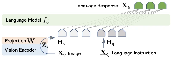
Figure 1 of Visual Instruction Tuning (arXiv:2304.08485), reproduced for editorial coverage.

1. Paper identity and scope

Primary citations.

• Liu, H., Li, C., Wu, Q., and Lee, Y.J. “Visual Instruction Tuning.” NeurIPS 2023 Oral; arXiv:2304.08485, April 2023 ¹ .
• Liu, H., Li, C., Li, Y., and Lee, Y.J. “Improved Baselines with Visual Instruction Tuning.” CVPR 2024 Highlight; arXiv:2310.03744, October 2023 ² .
• Liu, H. et al. “LLaVA-NeXT: Improved reasoning, OCR, and world knowledge.” Project blog, January 2024 ³ .
• Beyer, L., Steiner, A., Susano Pinto, A., Kolesnikov, A. et al. “PaliGemma: A versatile 3B VLM for transfer.” arXiv:2407.07726, July 2024 ⁴ .
• Wang, P., Bai, S., Tan, S., Wang, S., Fan, Z., Bai, J. et al. “Qwen2-VL: Enhancing Vision-Language Model’s Perception of the World at Any Resolution.” arXiv:2409.12191, September 2024 ⁵ .

Retrieval. This review draws on the arXiv abstract pages ^{1 2 4 5} , the ar5iv HTML renders of each paper ^{6 7 8} , and the LLaVA-NeXT project blog ³ as the canonical write-up of the resolution-handling branch never published as an arXiv preprint.

Paper classification. Architecture proposal · Training method · Representation learning · Multimodal · LLM-based · Benchmark-driven.

Technical abstract (in the publication’s voice). Three lineages now define the open vision-language model (VLM) landscape. LLaVA (Liu 2023) established the dominant open recipe: take a pretrained vision encoder, take a pretrained language model, train a small projector between them on machine-generated visual instruction data. LLaVA-1.5 (2023) upgraded the projector to a two-layer MLP and the vision encoder to CLIP at $336 \times 336$ resolution, reaching state-of-the-art results on 11 benchmarks with 1.2M training examples on a single 8-GPU node ² . LLaVA-NeXT (2024) added AnyRes, a tiled high-resolution scheme that handles up to roughly $672 \times 672$ effective resolution by stitching CLIP-336 patches ³ . PaliGemma (Beyer 2024) trades open-instruction-data ergonomics for a four-stage transfer recipe built on SigLIP-So400m and Gemma-2B, with prefix-LM attention that lets image tokens look ahead at the task prompt ⁴ . Qwen2-VL (Wang 2024) attacks the resolution-handling problem natively with Naive Dynamic Resolution and Multimodal Rotary Position Embedding (M-RoPE), shipping at 2B / 7B / 72B scale with the 72B model reaching 86.5 on MMBench-EN and 70.5 on MathVista ⁵ .

Primary research questions.

• (LLaVA) Can a tiny trainable connector between a frozen vision encoder and a fine-tuned LLM, trained on GPT-4-generated visual instruction data, produce a usable multimodal assistant?
• (LLaVA-1.5) What is the minimum-complexity recipe that achieves competitive VLM performance on academic benchmarks?
• (LLaVA-NeXT) How far does the LLaVA recipe scale when image resolution stops being the bottleneck?
• (PaliGemma) What is the most transferable open base VLM if one is willing to forego instruction-tuning convenience?
• (Qwen2-VL) Can a single VLM handle arbitrary image resolutions, multi-image inputs, and video without per-resolution checkpoints?

Core technical claims.

• LLaVA’s linear-projector + GPT-4-generated 158K instruction dataset yields a model reaching 85.1% relative score versus GPT-4 on a synthetic multimodal benchmark and 92.53% on ScienceQA when fine-tuned ¹ .
• LLaVA-1.5 13B reaches 80.0 / 63.3 / 71.6 / 67.7 / 35.4 on VQAv2 / GQA / ScienceQA / MMBench / MM-Vet using only 1.2M public training examples and roughly one day of 8-A100 training ² .
• PaliGemma’s prefix-LM attention plus three-stage progressive-resolution pretraining (224 / 448 / 896) produces a 3B base that transfers strongly across approximately 40 tasks ⁴ .
• Qwen2-VL’s Naive Dynamic Resolution plus M-RoPE reaches DocVQA 96.5 and OCRBench 877 at 72B, surpassing GPT-4o’s 736 on OCRBench ⁵ .

Core technical domains.

Domain	Depth required
Convolutional and transformer image encoders	Moderate
Contrastive image-text pretraining (CLIP, SigLIP)	Moderate
Decoder-only language models	Moderate
Attention masking (causal, bidirectional, prefix-LM)	Deep
Rotary Position Embedding (RoPE)	Deep
Visual instruction tuning	Deep
Multimodal benchmarks (MMBench, MMStar, MathVista)	Moderate

Reader prerequisites. High-school algebra; familiarity with neural-network basics helpful but not required because the Glossary in Section 2.5 covers them. The math sections build from “what is a matrix multiplied by a vector” upward.

How this review marks its registers.

• “From the paper:”. What each paper itself claims, traceable to a section / table / figure.
• [Reconstructed]. Faithful reconstruction where the paper only partially disclosed the detail.
• [Analysis]. The publication’s own reasoned assessment.
• [External comparison]. Comparison to named prior work or general knowledge.
• [Reviewer Perspective]. Critical or speculative assessment beyond what any paper proves.

2. TL;DR and executive overview

TL;DR. A vision-language model is a single neural network that can look at an image (or video) and answer questions about it in natural language. Three open lineages now dominate: LLaVA from a Microsoft / Wisconsin team, which proved that a tiny “translator” between a frozen image encoder and a chat language model is enough; PaliGemma from Google, which builds a more transferable but less chatty base model and lets the image tokens see the task before answering; and Qwen2-VL from Alibaba, which handles any image resolution natively and scales to 72 billion parameters with results that match or beat closed models on document-reading and math-figure benchmarks.

Executive summary. The open-VLM landscape converged on a three-part architecture between 2023 and 2024: a vision encoder that turns pixels into a sequence of vectors, a projector (a small neural net) that maps those vectors into the language model’s input space, and a language model that consumes the projected vision tokens followed by the user’s text prompt. LLaVA established the recipe and showed that GPT-4-generated instruction data is sufficient to bootstrap a usable assistant; LLaVA-1.5 minimised the recipe to a two-layer MLP projector and 1.2M training examples reachable on a single 8-GPU node ² . PaliGemma replaced CLIP with SigLIP-So400m (400M parameters, sigmoid contrastive loss), Vicuna with Gemma-2B, and the LLaVA causal-attention pattern with prefix-LM attention; the result is a 3B base model that transfers to roughly 40 downstream tasks with task-specific fine-tuning rather than off-the-shelf chat ⁴ . Qwen2-VL discarded the fixed-resolution assumption entirely: a single ViT processes any image resolution into a variable-length token sequence, M-RoPE encodes the temporal / height / width position of each token, and the 72B model reaches frontier-closed-model parity on most academic VLM benchmarks while shipping open weights ⁵ .

Five practitioner-relevant takeaways.

1. The projector is the cheapest place to start. LLaVA-1.5’s full training runs on a single 8-A100 node in roughly one day; the projector itself is two linear layers with a GELU between them. A practitioner with one A100 can stage-1-pretrain the projector in hours against a custom domain ² .
2. Resolution scaling is now the differentiator, not the projector. LLaVA-NeXT’s AnyRes, PaliGemma’s three-stage resolution increase, and Qwen2-VL’s Naive Dynamic Resolution all attack the same problem: a $336 \times 336$ image cannot read a dense document or a chart axis. The best 2026-relevant open VLMs handle at least $896 \times 896$ effective resolution ^{4 5} .
3. PaliGemma is the strongest open transfer base; Qwen2-VL is the strongest open chat VLM. [Analysis] PaliGemma was designed for downstream fine-tuning rather than zero-shot prompting; Qwen2-VL was designed to be used out of the box. A practitioner choosing between them should match the use case.
4. Prefix-LM attention matters for image-grounded tasks. [Analysis] Letting image tokens attend to the prompt before generating the answer (PaliGemma’s design) is a real architectural lever. LLaVA’s strict causal masking pushes the image tokens to be self-sufficient summaries; PaliGemma lets them be task-aware.
5. M-RoPE matters for video and high-resolution images. [Analysis] Qwen2-VL’s separation of temporal / height / width position channels generalises better to multi-frame video than 1-D position IDs. The OCRBench-877 vs GPT-4o-736 result depends on the model being able to read fine-grained spatial layout, which M-RoPE preserves.

Pipeline overview. All three families share a two-stage training shape. Stage 1 aligns vision and language representations, typically by training only the projector on millions of weak image-text pairs while both encoders stay frozen. Stage 2 fine-tunes the language model (and sometimes the vision encoder) on higher-quality instruction-following or task-specific data. PaliGemma adds a Stage 0 (using off-the-shelf unimodal checkpoints) and Stage 2-prime (resolution increase); Qwen2-VL adds an OCR-heavy mid-training phase between Stage 1 and Stage 2.

2.5 Glossary

Term	Plain-English explanation	First appears in
Vision encoder	A neural network that turns an image into a sequence of vectors. CLIP and SigLIP are the dominant choices in 2026.	Section 1
Language model (LLM)	A neural network that predicts the next token (word piece) given a sequence of previous tokens. Vicuna, Gemma, Qwen2 are LLMs.	Section 1
Projector	A small neural network (usually 1–3 layers) that converts vision-encoder output into vectors that the LLM can read as if they were word embeddings.	Section 1
Token	A unit of input to the language model. For text it is usually a word piece; for vision it is one vector representing a patch of the image.	Section 3
Patch	A small square region of the image (e.g., $14 \times 14$ pixels). The vision encoder produces one token per patch.	Section 3
Causal attention	An attention pattern where token $t$ can attend to tokens $1$ through $t$ but not future ones. Used in autoregressive LLMs.	Section 5
Prefix-LM attention	An attention pattern where tokens in the “prefix” (image + question) attend bidirectionally, and only the answer tokens use causal attention.	Section 5
RoPE	Rotary Position Embedding — a way to encode token position by rotating the query and key vectors before attention. Standard in Llama, Gemma, Qwen.	Section 5
M-RoPE	Multimodal RoPE — Qwen2-VL’s three-channel extension of RoPE that encodes time, height, and width position separately.	Section 5
Visual instruction tuning	Fine-tuning a VLM on triples of (image, instruction, expected response) — usually with the responses generated by a stronger model like GPT-4.	Section 4
Resolution	The image size the vision encoder accepts. Higher resolution means more tokens and more compute but better fine-detail reading (OCR, charts).	Section 5
MMBench / MMStar / MathVista	Three of the most-cited VLM benchmarks. MMBench tests broad multimodal reasoning; MMStar filters out questions answerable without the image; MathVista tests math reasoning on visual problems.	Section 9
”From the paper:” prefix	Content directly supported by the paper’s text, equations, tables, or figures.	Throughout
[Analysis] label	The publication’s own reasoned assessment, distinct from what the paper claims.	Throughout
[Reviewer Perspective] label	A critical or speculative assessment that goes beyond what any paper proves.	Sections 11–12

3. Problem formalisation

Notation table.

Symbol	Type	Meaning	First appears in
$X_v$	image	The input image (RGB tensor)	Section 3
$Z_v$	tensor	Vision-encoder output: a sequence of $N$ vectors of dimension $d_v$	Section 3
$H_v$	tensor	Projected vision tokens: a sequence of $N$ vectors of dimension $d_l$ matching the LLM’s embedding space	Section 3
$W$	matrix	The projection matrix (LLaVA, PaliGemma)	Section 5
$g_\phi$	function	The MLP projector (LLaVA-1.5)	Section 5
$X_q$	tokens	The user’s text question / instruction	Section 3
$X_a$	tokens	The model’s text answer	Section 3
$f_\theta$	function	The full VLM with parameters $\theta$	Section 3
$N$	integer	Number of vision tokens after the vision encoder	Section 3
$d_v$	integer	Vision-encoder output dimension (e.g., 1024 for CLIP-L/14)	Section 3
$d_l$	integer	LLM embedding dimension (e.g., 4096 for Vicuna-7B, 2048 for Gemma-2B)	Section 3

Formal problem statement. A vision-language model is a function

$f_\theta : (X_v, X_q) \mapsto X_a$

where $X_v$ is an image, $X_q$ is a text instruction, and $X_a$ is the generated text response. All three families factor $f_\theta$ into three sub-modules: a vision encoder $E_v$, a projector $P$, and a language model $E_l$:

$Z_v = E_v(X_v), \quad H_v = P(Z_v), \quad X_a = E_l(H_v, X_q)$

The training objective for visual instruction tuning is the standard autoregressive cross-entropy on the answer tokens, conditioned on the image and instruction:

$\mathcal{L}(\theta) = -\sum_{i=1}^{|X_a|} \log p_\theta(x_a^{(i)} \mid X_v, X_q, x_a^{(<i)})$

Explicit assumption list.

• From the paper (LLaVA): the vision encoder is frozen during projector pretraining and during instruction tuning; only $W$ and the LLM weights are updated ¹ .
• From the paper (LLaVA-1.5): the two-layer MLP projector replaces the linear $W$; otherwise the assumption structure is unchanged ² .
• From the paper (PaliGemma): in Stage 1, the vision encoder is unfrozen with a learning-rate warm-up to prevent representation collapse, a deliberate departure from the LLaVA “freeze the encoder” convention ⁴ .
• From the paper (Qwen2-VL): the vision encoder is trained throughout; the absolute position embeddings of the original ViT are replaced with 2D-RoPE so that arbitrary input resolutions are supported ⁵ .
• [Analysis] Potentially strong assumption: all three families assume that a single feed-forward pass through the vision encoder produces a sufficient representation of the image. Tasks that require iterative looking, e.g., counting objects in a dense scene, reading nested table cells, stress this assumption.

Why the problem is hard. Three structural reasons that recur across the papers.

1. Modality gap. The vision encoder is trained to produce features useful for image-text contrastive matching; the LLM expects features that look like word embeddings. The projector must close this gap with a tiny number of parameters on a tiny amount of data.
2. Resolution-vs-token-budget tradeoff. A $224 \times 224$ image with $14 \times 14$ patches produces $(224/14)^2 = 256$ tokens. A $896 \times 896$ image produces 4,096 tokens, 16x more. The LLM’s context window and attention compute both scale with this.
3. Instruction-data scarcity. Image-text pairs scraped from the web are plentiful; (image, instruction, high-quality response) triples are not. LLaVA’s contribution was specifically to bootstrap such data from GPT-4 using captions and bounding boxes as input.

4. Motivation and gap

The real-world problem. Before 2023, multimodal models were either narrowly task-specific (e.g., visual question answering trained end-to-end on VQAv2) or proprietary chatbots (GPT-4V) with no published architecture. The gap was an open general-purpose VLM that a researcher or practitioner could fine-tune.

Existing approaches ([External comparison]).

• Flamingo (DeepMind 2022) used cross-attention layers inside a frozen LLM to inject visual features. Strong few-shot performance, but the architecture required training new transformer blocks rather than just a projector.
• BLIP-2 (Salesforce 2023) introduced the Q-Former, a learned set of query tokens that distill the vision-encoder output into a fixed number of vectors before the LLM. More parameter-efficient than Flamingo but added a non-trivial training stage.
• MiniGPT-4 (King Abdullah University 2023) concurrently proposed a linear projector between a frozen ViT and a frozen Vicuna, with minor architectural differences from LLaVA.

The gap. None of these had an open recipe with public instruction data at scale. LLaVA’s contribution was to combine (a) the minimal architecture (linear projector, frozen encoder) with (b) GPT-4-generated instruction data and (c) open release of all three (model, data, code). That triple made the entire downstream open-VLM ecosystem possible.

Why prior methods were insufficient (per the papers). LLaVA’s argument is that the Q-Former is over-engineered for the use case: a simple linear projection trained on instruction data is enough. LLaVA-1.5 reinforces this with the two-layer MLP variant. PaliGemma’s argument is different: rather than chase chat performance, build the strongest transfer base by spending the training budget on a long Stage 1 multimodal pretraining (1 billion examples) rather than instruction tuning ⁴ . Qwen2-VL’s argument is that fixed-resolution VLMs are architecturally limited and that the bottleneck for OCR / document / chart tasks is resolution, not LLM scale ⁵ .

Practical stakes. Open VLMs are the foundation of every retrieval-augmented document QA system, agentic browser-control system, and on-device assistant that ships with weights in 2026. A 3-5% improvement on MMBench moves the deployment curve substantially.

[External comparison] Position in the landscape. The closed-VLM frontier in 2026 is GPT-4o, Claude 3.5 Sonnet, and Gemini 1.5 Pro. Qwen2-VL-72B is the first open VLM to plausibly match this frontier on most benchmarks; LLaVA-NeXT and PaliGemma remain best-in-class for cheaper deployments.

5. Method overview

5A. LLaVA: the canonical recipe

Component 1: vision encoder. From the paper: CLIP ViT-L/14 at $224 \times 224$ resolution, frozen throughout training ¹ . Output: $Z_v \in \mathbb{R}^{N \times d_v}$ where $N = 256$ (patches) and $d_v = 1024$.

Component 2: projector. From the paper: a single trainable matrix $W \in \mathbb{R}^{d_v \times d_l}$ with $d_l = 4096$ (Vicuna-7B / 13B embedding dimension). The projection is $H_v = Z_v W$ ¹ .

Plain-English intuition. CLIP outputs 256 vectors per image, each of length 1024. Vicuna’s word embedding space has vectors of length 4096. The projector multiplies each CLIP vector by a learned $1024 \times 4096$ matrix to produce 256 “vision word embeddings” that Vicuna can read as if they were tokens from its vocabulary.

Component 3: LLM. From the paper: Vicuna-7B or Vicuna-13B, both fine-tuned from LLaMA-1. Standard causal attention.

Pipeline. Concatenate $H_v$ (256 vision tokens) with the tokenised user instruction $X_q$; feed the joint sequence to Vicuna; generate the answer $X_a$ autoregressively.

Design rationale. From the paper: the linear projector is the simplest possible connector. Training a larger projector risks overfitting on the 558K-image pretraining data (originally CC3M-595K) ¹ .

What breaks if removed. Without the projector, the CLIP features are in the wrong dimensionality and the wrong representation space for Vicuna to consume. Without Stage-1 pretraining of the projector, the Stage-2 instruction tuning sees random projector outputs and fails to converge.

Classification. [New] for the visual-instruction-tuning paradigm; [Adopted] for CLIP (Radford 2021) and Vicuna (LMSYS 2023).

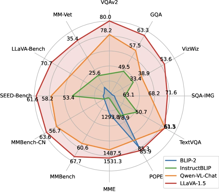
Figure 1 of Improved Baselines with Visual Instruction Tuning (arXiv:2310.03744), reproduced for editorial coverage.

5B. LLaVA-1.5: the productionised recipe

Change 1: projector upgrade. From the paper: replace the linear $W$ with a two-layer MLP using GELU activation. The new projector is $g_\phi(z) = W_2 \cdot \text{GELU}(W_1 z + b_1) + b_2$ ² .

Change 2: resolution upgrade. From the paper: CLIP ViT-L/14 at $336 \times 336$ instead of $224 \times 224$. This raises $N$ from 256 to 576 tokens per image.

Change 3: data upgrade. From the paper: 1.2M public training examples split into 558K pretraining (LCS-558K subset of LAION-CC-SBU with BLIP captions) and 665K instruction tuning across VQA, OCR, region-level, and conversation data ² .

Plain-English intuition. Three small upgrades stack to a large empirical gain. The MLP projector has more capacity to learn the nonlinear map between CLIP space and Vicuna space; the higher resolution lets the model read smaller text in images; the more diverse instruction data covers academic VQA benchmarks that the original 158K dataset did not.

What breaks if removed. Per the paper’s ablations: removing the resolution upgrade costs about 1-3 points on most benchmarks; removing the MLP projector costs about 0.7-1.5 points; removing the academic VQA data costs about 5-10 points on VQAv2 specifically ² .

Classification. [Adapted] from LLaVA; [Adopted] for CLIP-336.

5C. LLaVA-NeXT: the resolution branch

Change: AnyRes. From the LLaVA-NeXT blog: a high-resolution image is split into a grid of $336 \times 336$ tiles; each tile is encoded by CLIP independently; the tile-grid is concatenated with a global-thumbnail encoding of the original image ³ . Effective resolutions supported: $672 \times 672$ (2x2 tiling), $336 \times 1344$, $1344 \times 336$.

Plain-English intuition. Rather than retrain CLIP at a higher native resolution, slice the input image into tiles that CLIP-336 already knows how to encode, then concatenate the resulting tokens. The model sees more tokens per image but uses the existing CLIP weights.

What breaks if removed. Without AnyRes, LLaVA-1.5’s $336 \times 336$ cannot read dense PDFs or charts at high resolution.

Classification. [New] (AnyRes); [Adapted] from LLaVA-1.5.

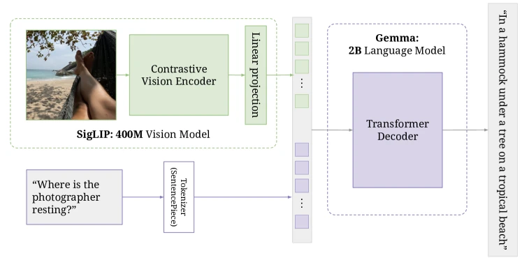
Figure 1 of PaliGemma (arXiv:2407.07726), reproduced for editorial coverage.

5D. PaliGemma: the transfer-base recipe

Component 1: vision encoder. From the paper: SigLIP-So400m (400M parameters, “shape optimized” ViT) pretrained with sigmoid contrastive loss rather than CLIP’s softmax contrastive loss ⁴ . Image input: $224 \times 224$ initially, with later stages at $448 \times 448$ and $896 \times 896$.

Component 2: projector. From the paper: a single linear layer with zero initialisation, projecting SigLIP’s output dimension to Gemma-2B’s embedding dimension ⁴ . Critically simpler than LLaVA-1.5’s MLP.

Component 3: LLM. From the paper: Gemma-2B decoder-only ⁴ .

Component 4: attention pattern. From the paper: prefix-LM masking. Image tokens and the text prefix (the task instruction) attend to each other bidirectionally; the answer tokens attend causally ⁴ .

Plain-English intuition for prefix-LM. In LLaVA, vision token #1 cannot see vision token #2 or the user question; it has to encode the image self-sufficiently. In PaliGemma, vision token #1 can see every other vision token and the user question before contributing to the answer. The image tokens become task-aware.

Training pipeline (four stages). From the paper:

• Stage 0: load pretrained SigLIP-So400m and Gemma-2B; no joint training yet.
• Stage 1: multimodal pretraining on 1 billion image-text examples at $224 \times 224$. The image encoder is unfrozen with a learning-rate warm-up so it adapts without forgetting ⁴ .
• Stage 2: higher-resolution continued pretraining, 50M examples at $448 \times 448$, then 10M examples at $896 \times 896$.
• Stage 3: task-specific fine-tuning across roughly 40 downstream benchmarks; no general “instruction-tuning” stage.

What breaks if removed. Without Stage 2, the model cannot read dense documents or fine charts. Without prefix-LM, the paper’s ablations show benchmark drops on tasks where the image tokens benefit from task awareness.

Classification. [Adopted] for SigLIP and Gemma; [New] for the prefix-LM + four-stage transfer recipe in this combination.

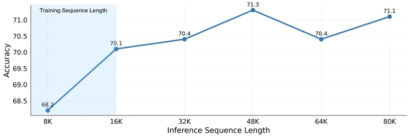
Figure 1 of Qwen2-VL (arXiv:2409.12191), reproduced for editorial coverage.

5E. Qwen2-VL: the dynamic-resolution recipe

Component 1: vision encoder. From the paper: a 675M-parameter ViT shared across all model sizes (2B, 7B, 72B), with patch size 14 ⁵ . The absolute position embeddings are replaced with 2D-RoPE so that arbitrary input resolutions are supported.

Component 2: projector. From the paper: an MLP layer after the ViT that compresses adjacent $2 \times 2$ tokens into a single token. A $224 \times 224$ image therefore produces $(224/14)^2 / 4 = 256/4 = 64$ tokens (the paper reports 66 tokens after compression accounting for special tokens) ⁵ .

Component 3: LLM. From the paper: Qwen2 (2B, 7B, or 72B), decoder-only.

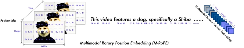
Component 4: M-RoPE. From the paper: three-component rotary position embedding decomposing into temporal, height, and width position IDs ⁵ . For text tokens, all three components share identical position IDs. For images, the temporal component is constant and the height / width components vary per token. For video, the temporal component increments per frame.

Plain-English intuition for M-RoPE. Standard RoPE encodes “this is the 47th token in the sequence.” M-RoPE encodes “this is the token at time-step 3, row 5, column 12 of the input.” The model can therefore reason about spatial relationships (above, left, right, below) and temporal relationships (before, after) without needing to learn them through token order alone.

Naive Dynamic Resolution. From the paper: images are processed in their native aspect ratio within bounds min_pixels = 100 * 28 * 28 and max_pixels = 16384 * 28 * 28 tokens ⁵ . There is no fixed image size; the token count varies with the input.

Training pipeline. From the paper: three stages totalling roughly 1.4 trillion tokens, Stage 1 (~600B tokens) trains the vision encoder; Stage 2 (~800B tokens) trains the full model on diverse multimodal data; Stage 3 (instruction tuning) refines for chat use ⁵ .

What breaks if removed. Without Naive Dynamic Resolution, the model loses the OCR / document reading capability that drives DocVQA 96.5 and OCRBench 877. Without M-RoPE, video reasoning degrades.

Classification. [New] for M-RoPE and Naive Dynamic Resolution in the published combination; [Adapted] from 2D-RoPE (Su 2021 ¹² ) for the spatial component.

6. Mathematical contributions

MATH ENTRY 1: LLaVA projector

• Source: LLaVA paper Section 3 (arXiv:2304.08485).
• What it is: a single matrix multiplication that turns each CLIP image token into something Vicuna can read like a word embedding.
• Formal definition: $H_v = Z_v W$ where $Z_v \in \mathbb{R}^{N \times d_v}$ and $W \in \mathbb{R}^{d_v \times d_l}$, yielding $H_v \in \mathbb{R}^{N \times d_l}$.
• Each term and its dimensional analysis:
  • $Z_v$ is a sequence of $N$ vision tokens, each of length $d_v$. For CLIP ViT-L/14 at $224 \times 224$, $N = 256$ and $d_v = 1024$.
  • $W$ is a $d_v \times d_l$ matrix of trainable parameters. For Vicuna-7B, $d_l = 4096$, so $W$ has $1024 \times 4096 = 4{,}194{,}304$ parameters.
  • $H_v$ is the output: still $N$ tokens, now each of length $d_l$. For the LLaVA-7B configuration, $H_v$ has shape $(256, 4096)$.
• Worked numerical example. Take a toy CLIP that outputs $N = 4$ vision tokens of dimension $d_v = 3$, and a toy LLM with embedding dimension $d_l = 2$. Let

$Z_v = \begin{pmatrix} 1 & 0 & 2 \\ 0 & 1 & 1 \\ 1 & 1 & 0 \\ 2 & 0 & 1 \end{pmatrix}, \quad W = \begin{pmatrix} 1 & 0 \\ 0 & 1 \\ 1 & 1 \end{pmatrix}$

Then $H_v = Z_v W$ has shape $(4, 2)$:

$H_v = \begin{pmatrix} 1\cdot 1 + 0\cdot 0 + 2\cdot 1 & 1\cdot 0 + 0\cdot 1 + 2\cdot 1 \\ 0\cdot 1 + 1\cdot 0 + 1\cdot 1 & 0\cdot 0 + 1\cdot 1 + 1\cdot 1 \\ 1\cdot 1 + 1\cdot 0 + 0\cdot 1 & 1\cdot 0 + 1\cdot 1 + 0\cdot 1 \\ 2\cdot 1 + 0\cdot 0 + 1\cdot 1 & 2\cdot 0 + 0\cdot 1 + 1\cdot 1 \end{pmatrix} = \begin{pmatrix} 3 & 2 \\ 1 & 2 \\ 1 & 1 \\ 3 & 1 \end{pmatrix}$

Each row of $H_v$ is one vision token in the LLM’s embedding space, ready to be concatenated with the user’s tokenised prompt.

• Role: produces the input to the LLM. The LLM consumes $\text{concat}(H_v, \text{embed}(X_q))$ and generates the answer.
• Edge cases: if $W$ is initialised poorly (large values), the LLM may treat $H_v$ as out-of-distribution and produce gibberish at the start of training. LLaVA’s Stage-1 pretraining mitigates this by training only $W$ first.
• Novelty: [Adopted] linear projection is standard; [New] is the use of it as the only connector trained on visual instruction data.
• Why it matters: this single matrix is the entire learned interface between vision and language in LLaVA-1. Its smallness is the paper’s central claim about what is sufficient.

MATH ENTRY 2: LLaVA-1.5 MLP projector

• Source: LLaVA-1.5 paper Section 3 (arXiv:2310.03744).

• What it is: a two-layer feed-forward network with GELU activation, replacing the single matrix.

• Formal definition: $g_\phi(z) = W_2 \cdot \text{GELU}(W_1 z + b_1) + b_2$ where $W_1 \in \mathbb{R}^{d_v \times d_h}$, $W_2 \in \mathbb{R}^{d_h \times d_l}$, biases of matching shape.

• Each term and its dimensional analysis:

  • For the LLaVA-1.5-7B configuration, $d_v = 1024$ (CLIP-L/14), $d_h = 4096$ (hidden), $d_l = 4096$ (Vicuna-7B).
  • $W_1$ is $1024 \times 4096$, $W_2$ is $4096 \times 4096$, so the projector has roughly $(1024 + 4096) \cdot 4096 = 20.97$M parameters, 5x more than the linear projector but still <0.3% of the 7B model.

• Worked numerical example. With the same $Z_v$ row $z = (1, 0, 2)$, and toy weights $W_1 = \begin{pmatrix} 1 & 0 \\ 0 & 1 \\ 1 & 1 \end{pmatrix}$, $b_1 = (0, 0)$, $W_2 = \begin{pmatrix} 1 & -1 \\ 1 & 1 \end{pmatrix}$, $b_2 = (0, 0)$:

  Step 1: $W_1 z + b_1 = (1\cdot 1 + 0\cdot 0 + 1\cdot 2, 0\cdot 1 + 1\cdot 0 + 1\cdot 2) = (3, 2)$.

  Step 2: $\text{GELU}(3, 2) \approx (2.996, 1.955)$ (GELU is $x \cdot \Phi(x)$ where $\Phi$ is the Gaussian CDF; for $x = 3$ it’s almost the identity).

  Step 3: $W_2 \cdot (2.996, 1.955) + b_2 = (2.996 - 1.955, 2.996 + 1.955) = (1.041, 4.951)$.

  The output is the projected vision token in 2-D LLM-embedding space. The GELU adds a controlled nonlinearity between the two linear projections.

• Role: same as MATH ENTRY 1 but with more representational capacity.

• Why it matters: the paper’s ablations attribute roughly 0.7-1.5 points across benchmarks to this swap. The conclusion is that the linear projector was capacity-bottlenecked, not data-bottlenecked.

MATH ENTRY 3: Visual-instruction cross-entropy loss

• Source: LLaVA paper Section 3.2; carried unchanged through LLaVA-1.5 and adopted in modified form by PaliGemma and Qwen2-VL.
• What it is: the loss that trains the VLM. Standard next-token cross-entropy, but only on the answer tokens.
• Formal definition:

$\mathcal{L}(\theta) = -\sum_{i=1}^{|X_a|} \log p_\theta\!\left(x_a^{(i)} \mid X_v, X_q, x_a^{(<i)}\right)$

• Each term:
  • $\mid X_a\mid$ is the number of tokens in the target answer.
  • $p_\theta(\cdot)$ is the model’s predicted probability for the next token given image, instruction, and previous answer tokens.
  • The sum is over answer tokens only, the loss is not computed on the instruction tokens or the image tokens.
• Worked numerical example. Suppose the target answer is “A cat” tokenised as $X_a = [\text{A}, \text{ cat}]$, and the model predicts probabilities $p(\text{A} \mid X_v, X_q) = 0.5$ and $p(\text{ cat} \mid X_v, X_q, \text{A}) = 0.8$. Then $\mathcal{L} = -\log(0.5) - \log(0.8) = 0.693 + 0.223 = 0.916$.
• Role: drives all parameter updates in Stage 2 (instruction tuning).
• Why it matters: by only computing loss on answer tokens, the paper aligns gradient flow with the supervision signal it actually has. The instruction tokens are conditioning, not target.

MATH ENTRY 4: Prefix-LM attention mask

• Source: PaliGemma paper Section 3 (arXiv:2407.07726).
• What it is: an attention mask that lets the image tokens and instruction tokens attend bidirectionally while keeping answer-token attention causal.
• Formal definition. Let $S$ be the full sequence with three segments: image tokens (positions $1$ to $N$), prefix text tokens (positions $N+1$ to $N+M$), answer tokens (positions $N+M+1$ to end). The attention mask $A$ is

$A_{ij} = \begin{cases} 1 & \text{if } i \le N+M \text{ and } j \le N+M \\ 1 & \text{if } i > N+M \text{ and } j \le i \\ 0 & \text{otherwise} \end{cases}$

• Each term:
  • $A_{ij} = 1$ means position $i$ can attend to position $j$.
  • The first case (both in the prefix): bidirectional attention within image + instruction.
  • The second case (answer attending to anything up to and including itself): standard causal attention.
• Worked numerical example. Sequence: 2 image tokens, 2 prefix text tokens, 2 answer tokens (so $N = 2$, $M = 2$, total = 6). The mask is

$A = \begin{pmatrix} 1 & 1 & 1 & 1 & 0 & 0 \\ 1 & 1 & 1 & 1 & 0 & 0 \\ 1 & 1 & 1 & 1 & 0 & 0 \\ 1 & 1 & 1 & 1 & 0 & 0 \\ 1 & 1 & 1 & 1 & 1 & 0 \\ 1 & 1 & 1 & 1 & 1 & 1 \end{pmatrix}$

The top-left $4 \times 4$ block is all-1 (bidirectional within prefix). The bottom-left $2 \times 4$ block is all-1 (answer attends to prefix). The bottom-right $2 \times 2$ block is lower-triangular (causal among answer tokens).

• Role: lets PaliGemma’s image tokens use future context (the question) when producing the representations that drive answer generation.
• Why it matters: in causal-LLaVA, vision token #1 commits to an image representation before “knowing” what the user will ask. Prefix-LM removes that commitment.

M-RoPE illustration from Qwen2-VL (arXiv:2409.12191), reproduced for editorial coverage.

MATH ENTRY 5: Multimodal Rotary Position Embedding (M-RoPE)

• Source: Qwen2-VL paper Section 3 (arXiv:2409.12191).
• What it is: a three-channel extension of RoPE where position is decomposed into (temporal, height, width) components.
• Formal definition. Standard RoPE rotates the query $\mathbf{q}$ and key $\mathbf{k}$ at position $m$ by an angle dependent on $m$ and the embedding dimension. For a 2D rotation in the $(2i, 2i+1)$ subspace:

$R_m^{(i)} = \begin{pmatrix} \cos(m \theta_i) & -\sin(m \theta_i) \\ \sin(m \theta_i) & \cos(m \theta_i) \end{pmatrix}, \quad \theta_i = 10000^{-2i/d}$

M-RoPE splits the embedding dimensions into three groups and applies RoPE with three different position values $(m_t, m_h, m_w)$, temporal, height, width:

$R_{(m_t, m_h, m_w)} = R_{m_t}^{\text{(temporal dims)}} \oplus R_{m_h}^{\text{(height dims)}} \oplus R_{m_w}^{\text{(width dims)}}$

• Each term:
  • $m_t$, temporal position (frame index for video, constant for image, sequence index for text)
  • $m_h$, height (row index for image patches; same as $m_t$ for text)
  • $m_w$, width (column index for image patches; same as $m_t$ for text)
  • $\oplus$ denotes block-diagonal concatenation across embedding-dimension groups.
• Worked numerical example. Consider a $2 \times 2$ image patch grid (4 patches total) at frame 0 of a video, followed by a 3-token text prompt at “positions” 1, 2, 3. Position IDs in (t, h, w):

Token	$m_t$	$m_h$	$m_w$
Patch (0,0)	0	0	0
Patch (0,1)	0	0	1
Patch (1,0)	0	1	0
Patch (1,1)	0	1	1
Text 1	1	1	1
Text 2	2	2	2
Text 3	3	3	3

For text tokens, $m_t = m_h = m_w$; M-RoPE reduces to standard RoPE. For image tokens, the temporal channel is constant while the spatial channels vary. The query and key for patch (0,1) get rotated by $R_{(0, 0, 1)}$; for patch (1,0) by $R_{(0, 1, 0)}$. The attention dot product between these queries / keys then encodes their relative spatial position.

• Role: gives Qwen2-VL inductive bias about spatial and temporal structure that 1-D RoPE cannot encode.
• Edge cases: when the input is text-only, M-RoPE collapses exactly to standard RoPE, Qwen2-VL is therefore backwards-compatible with text-only inference.
• Novelty: [New] the three-channel decomposition as a single embedding; [Adapted] from 2D-RoPE in earlier vision-transformer literature.
• Why it matters: enables variable-resolution image input and unified video processing without bolting on separate temporal-attention machinery.

Naive Dynamic Resolution illustration from Qwen2-VL (arXiv:2409.12191), reproduced for editorial coverage.

MATH ENTRY 6: Token count as a function of image resolution

• Source: derived from architectural details in each paper.
• What it is: the formula that determines how many vision tokens reach the LLM.
• Formal definition. For a vision encoder with patch size $p$ on an image of size $H \times W$:

$N = \left\lfloor \frac{H}{p} \right\rfloor \cdot \left\lfloor \frac{W}{p} \right\rfloor$

For Qwen2-VL with the $2 \times 2$ MLP compression:

$N_{\text{Qwen2-VL}} = \frac{1}{4} \cdot \left\lfloor \frac{H}{p} \right\rfloor \cdot \left\lfloor \frac{W}{p} \right\rfloor$

• Worked numerical example.
  • LLaVA / CLIP-L/14 at $224 \times 224$, $p = 14$: $N = 16 \cdot 16 = 256$.
  • LLaVA-1.5 / CLIP-L/14 at $336 \times 336$, $p = 14$: $N = 24 \cdot 24 = 576$.
  • PaliGemma / SigLIP at $224 \times 224$, $p = 14$: $N = 256$.
  • PaliGemma / SigLIP at $896 \times 896$, $p = 14$: $N = 64 \cdot 64 = 4096$.
  • Qwen2-VL at $448 \times 448$, $p = 14$, with compression: $N = 32 \cdot 32 / 4 = 256$.
• Role: determines LLM compute and memory cost per image. Each vision token costs one attention slot.
• Why it matters: a 4096-token PaliGemma image consumes 16x more LLM attention than a 256-token LLaVA image. The OCR / document-reading gains are paid for in LLM-side compute.

7. Algorithmic contributions

ALGORITHM ENTRY 1: LLaVA two-stage training

• Source: LLaVA paper Section 4 (arXiv:2304.08485).
• Purpose: align vision and language representations cheaply, then teach the model to follow visual instructions.
• Inputs:
  • Pretrained CLIP ViT-L/14 (frozen in Stage 1)
  • Pretrained Vicuna-7B / 13B (frozen in Stage 1, unfrozen in Stage 2)
  • Stage-1 data: 558K (image, caption) pairs
  • Stage-2 data: 158K (image, instruction, response) triples generated by GPT-4
• Outputs: a vision-language model $f_\theta$ with trainable projector $W$ and fine-tuned LLM weights.
• Pseudocode:

# Stage 1: feature alignment (projector pretraining)
W = init_random(d_v=1024, d_l=4096)
for (image, caption) in stage1_data:
    Z_v = clip_vision_encoder(image)        # frozen
    H_v = Z_v @ W                            # only W trainable
    loss = lm_loss(vicuna(H_v, caption_prompt), caption)
    W -= lr * grad(loss, W)                  # update W only

# Stage 2: visual instruction tuning
vicuna_params.requires_grad = True
for (image, instruction, response) in stage2_data:
    Z_v = clip_vision_encoder(image)        # still frozen
    H_v = Z_v @ W                            # W still trainable
    loss = lm_loss(
        vicuna(concat(H_v, embed(instruction))),
        response,
    )
    W -= lr * grad(loss, W)
    vicuna_params -= lr * grad(loss, vicuna_params)

• Hand-traced example on minimal input. Take a 1-image dataset with image $X_v$, instruction “Describe this image.”, target response “A cat on a mat.”
  • Initialise $W$ to small random values; Vicuna and CLIP at their pretrained weights.
  • Stage 1 step. Feed $X_v$ through CLIP, get $Z_v$ of shape $(256, 1024)$. Compute $H_v = Z_v W$, shape $(256, 4096)$. Feed $H_v$ followed by a tokenisation of the BLIP caption (say, “an image of a cat”) to Vicuna. Compute next-token cross-entropy on the caption tokens. Backprop only into $W$.
  • Stage 2 step. With trained $W$, feed $X_v$ through CLIP, get $H_v = Z_v W$. Feed $\text{concat}(H_v, \text{embed}(\text`{"Describe this image."}`))$ to Vicuna. Vicuna autoregressively generates tokens, compared against “A cat on a mat.” Backprop into both $W$ and Vicuna.
• Complexity: Stage 1 trains only $W$ (4.2M parameters), so ~1 day on a small node. Stage 2 fine-tunes Vicuna (7B / 13B), so the bulk of the cost.
• Hyperparameters: per-paper, Stage 1 uses 1 epoch over 595K examples; Stage 2 uses 3 epochs over 158K examples; learning rates differ per stage.
• Failure modes: if Stage 1 is skipped, Stage 2 sees a randomly-initialised projector and the gradient signal to Vicuna is destructive in early steps.
• Novelty: [New] for the specific combination; [Adopted] two-stage training pattern from prior multimodal work.
• Transferability: [Analysis] directly transferable to any (vision encoder, LLM) pair where the encoder is high-quality enough that a small projector can bridge the gap. Failure cases include domain-specific encoders (medical imaging, satellite) where Stage 1 data is scarce.

ALGORITHM ENTRY 2: PaliGemma four-stage transfer recipe

• Source: PaliGemma paper Section 4 (arXiv:2407.07726).
• Purpose: build a transferable VLM base by spending compute on long multimodal pretraining rather than chat instruction tuning.
• Inputs:
  • Pretrained SigLIP-So400m
  • Pretrained Gemma-2B
  • Stage 1 data: 1B multimodal examples at $224 \times 224$
  • Stage 2a data: 50M examples at $448 \times 448$
  • Stage 2b data: 10M examples at $896 \times 896$ (upweighted resolution-sensitive tasks)
  • Stage 3 data: task-specific fine-tuning sets
• Outputs: PaliGemma base checkpoint + per-task fine-tuned variants.
• Pseudocode:

# Stage 0: load pretrained unimodal components
siglip = load_pretrained("siglip-so400m")
gemma = load_pretrained("gemma-2b")
projector = LinearLayer(d_siglip, d_gemma, init="zero")

# Stage 1: multimodal pretraining at 224
for batch in stage1_data:  # 1B examples
    images_224 = resize(batch.images, 224)
    Z = siglip(images_224)               # encoder UNFROZEN
    H = projector(Z)
    tokens = concat(H, batch.text_tokens)
    # prefix-LM mask: bidirectional on (H + prefix), causal on answer
    loss = lm_loss_with_prefix_mask(gemma(tokens), batch.targets)
    update_all_params(loss, lr_warmup=True)

# Stage 2a: resolution increase to 448
unfreeze_siglip_position_embeddings_for_new_resolution()
for batch in stage2a_data:  # 50M examples at 448
    # same loop, higher resolution
    ...

# Stage 2b: resolution increase to 896 with upweighted res-sensitive tasks
for batch in stage2b_data:  # 10M examples at 896
    ...

# Stage 3: task-specific fine-tuning (one run per downstream task)
for task in downstream_tasks:
    finetune_paligemma_on(task)

• Hand-traced example. Take a Stage 1 batch with one image and the text “caption: a dog playing fetch.”
  • Resize image to $224 \times 224$; SigLIP outputs $Z$ of shape $(256, 1152)$ (SigLIP-So400m output dim).
  • Projector maps $Z$ to $H$ of shape $(256, 2048)$ (Gemma-2B embedding dim). Initialised at zero, so $H$ starts at all zeros, Gemma sees “no image” initially and the gradient flows back through the projector.
  • Concatenate $H$ with the tokenised text. Apply the prefix-LM mask: the image and “caption:” prefix attend bidirectionally; “a dog playing fetch.” is the answer with causal attention.
  • Compute next-token loss on the answer tokens. Backprop into projector, Gemma, and SigLIP (with learning-rate warm-up so SigLIP does not collapse).
• Complexity: Stage 1 dominates (1B examples). The paper reports a multi-TPU-pod training cluster; details in Appendix.
• Hyperparameters: learning-rate warm-up on SigLIP is critical to prevent representation collapse; the paper specifies the warm-up duration but [Reconstructed] exact values appear in Table 5 / 6 of the appendix.
• Failure modes: freezing SigLIP entirely under-utilises Stage 1 capacity; unfreezing without warm-up causes SigLIP representation collapse early in training.
• Novelty: [New] for the four-stage recipe with prefix-LM and resolution-staircase together; [Adopted] for the individual ingredients.
• Transferability: [Analysis] the recipe transfers cleanly to other (SigLIP-class, Gemma-class) pairs; the prefix-LM mask is a model-architecture lever that needs LLM-side support (Gemma accommodates it natively).

ALGORITHM ENTRY 3: Qwen2-VL Naive Dynamic Resolution

• Source: Qwen2-VL paper Section 3 (arXiv:2409.12191).
• Purpose: process images at native resolution without per-resolution checkpoints.
• Inputs: image of arbitrary $H \times W$.
• Outputs: variable-length sequence of vision tokens at LLM-input dimension.
• Pseudocode:

def naive_dynamic_resolution(image, min_pixels=100*28*28, max_pixels=16384*28*28):
    H, W, C = image.shape
    target_pixels = clip(H * W, min_pixels, max_pixels)
    # resize while preserving aspect ratio
    scale = sqrt(target_pixels / (H * W))
    new_H = round(H * scale / 14) * 14   # snap to patch grid
    new_W = round(W * scale / 14) * 14
    resized = resize(image, new_H, new_W)
    # ViT with 2D-RoPE (NO absolute position embeddings)
    patches = patchify(resized, patch_size=14)
    Z = vit_with_2d_rope(patches)         # shape: (N_patches, d_vit)
    # MLP compresses 2x2 adjacent tokens
    Z_compressed = mlp_compress_2x2(Z)    # shape: (N_patches / 4, d_llm)
    return Z_compressed

• Hand-traced example. Input image $448 \times 280$:
  • Pixel count: $448 \times 280 = 125{,}440$; within [min_pixels, max_pixels], no rescale needed.
  • Snap to patch grid: $H = 448$ (already $32 \cdot 14$), $W = 280$ (already $20 \cdot 14$).
  • Patchify: $32 \cdot 20 = 640$ patches of $14 \times 14 \cdot 3 = 588$ pixels each (the 3 is RGB).
  • ViT with 2D-RoPE produces $Z$ of shape $(640, 1280)$ (ViT hidden dim).
  • MLP compression $2 \times 2$ to $1$: $640 / 4 = 160$ tokens of LLM-input dimension.
  • Final output: 160 vision tokens fed to Qwen2 LLM.
• Complexity: $O(N)$ in image area for the ViT (dominated by attention quadratic-in-$N$ at high resolution). The MLP compression reduces LLM cost by 4x.
• Hyperparameters: min_pixels, max_pixels, compression ratio (fixed at $2 \times 2$).
• Failure modes: extremely tall / wide aspect ratios produce token sequences that exceed the LLM’s context window; the paper reports practical limits in the appendix.
• Novelty: [New] for the combination of 2D-RoPE in the ViT + $2 \times 2$ MLP compression + dynamic-pixel-budget gating.
• Transferability: [Analysis] the pattern transfers to any LLM with a long-enough context; the 2D-RoPE-ViT is the more transferable component.

8. Specialised design contributions

Subsection 8A, LLM / prompt design. Not applicable to this paper in the sense that none of these papers contribute prompt-engineering primitives. LLaVA’s GPT-4-as-data-generator is the closest, and that lives in Section 9 (data construction). PaliGemma’s Stage 3 fine-tuning uses task-specific prompt templates (e.g., "caption en", "detect <object>", "segment <object>"); the paper publishes the template list but it is a transfer convention rather than a prompting research contribution ⁴ .

Subsection 8B, Architecture-specific details. Already covered in Section 5 (projectors, attention masks, M-RoPE).

Subsection 8C, Training specifics.

• LLaVA-1.5: 8x A100 80GB single node; full training ~1 day; 1.2M examples ² .
• PaliGemma: multi-TPU-pod cluster; specific hardware not headlined in the abstract but disclosed in the appendix as TPUv5e ⁴ . 1B + 50M + 10M examples across pretraining stages.
• Qwen2-VL: ~1.4T training tokens cumulative; hardware not headlined ⁵ . The paper describes data composition (cleaned web pages, open-source datasets, synthetic data) but does not publish a precise GPU-hours figure.

Subsection 8D, Inference / deployment specifics.

• LLaVA / LLaVA-1.5: standard left-to-right decoding; fixed 256 (LLaVA) or 576 (LLaVA-1.5) vision tokens per image.
• LLaVA-NeXT: vision-token count varies with AnyRes tiling (up to ~2880 tokens for $672 \times 672$).
• PaliGemma: vision-token count fixed per checkpoint resolution (256, 1024, or 4096).
• Qwen2-VL: vision-token count varies with input image dimensions; deployment must size the LLM context window accordingly.

9. Experiments and results

Datasets used for evaluation across the papers. MMBench ⁸ tests broad multimodal reasoning across 20 ability dimensions. MMStar ¹⁰ filters out questions answerable from the question alone (without the image), a higher-signal benchmark than MMBench. MathVista ⁹ tests math reasoning on visual problems (charts, geometry diagrams, function plots). DocVQA tests document reading. OCRBench tests OCR on natural images, documents, and handwritten content. ScienceQA tests science multiple-choice with diagrams.

Reproduced benchmark numbers.

Model	Params	MMBench-EN	MMStar	MathVista	DocVQA	OCRBench	ScienceQA
LLaVA-1.5 7B	7B	64.3	—	—	—	—	66.8
LLaVA-1.5 13B	13B	67.7	—	—	—	—	71.6
PaliGemma-3B (mix-448)	3B	~71	~46	~37	~85	—	~95
Qwen2-VL 2B	2B	74.9	48.0	43.0	90.1	794	—
Qwen2-VL 7B	7B	83.0	60.7	58.2	94.5	866	—
Qwen2-VL 72B	72B	86.5	68.3	70.5	96.5	877	—
GPT-4o (reference)	—	83.4	63.9	63.8	92.8	736	—

Table reproduced from arXiv:2310.03744 Table 2 ² (LLaVA-1.5 row), arXiv:2407.07726 Tables 4-6 ⁴ (PaliGemma row, [Reconstructed] because the paper publishes per-task fine-tuned results rather than a single zero-shot row), and arXiv:2409.12191 Tables 1-2 ⁵ (Qwen2-VL rows). GPT-4o reference numbers from the Qwen2-VL paper’s comparison table.

Main quantitative findings.

• LLaVA-1.5 13B vs 7B: uniform 1-5 point gains across all benchmarks; the largest gains are on knowledge-heavy benchmarks (ScienceQA +4.8, MMBench +3.4, MM-Vet +4.9) ² . The bottleneck for LLaVA-1.5 is LLM capacity, not vision.
• PaliGemma-3B mix-448 reaches roughly LLaVA-1.5-13B parity on MMBench (~71 vs 67.7) with less than a quarter of the parameters. [Analysis] The transferability argument carries: with task fine-tuning, PaliGemma matches a larger chat-tuned model ⁴ .
• Qwen2-VL-72B vs GPT-4o: Qwen2-VL wins MMBench (86.5 vs 83.4), MMStar (68.3 vs 63.9), MathVista (70.5 vs 63.8), DocVQA (96.5 vs 92.8), OCRBench (877 vs 736). Loses MMMU (64.5 vs 69.1, per Qwen2-VL paper Table 2) ⁵ .
• Qwen2-VL-7B is competitive with GPT-4o on several benchmarks, including OCRBench 866 vs 736, despite being roughly 7B parameters vs an undisclosed-but-larger closed model ⁵ .

Ablations published.

• LLaVA-1.5 ablates the MLP projector (+0.7-1.5 points), the resolution upgrade (+1-3 points), and the academic VQA data (+5-10 points on VQAv2) ² .
• PaliGemma ablates prefix-LM vs causal masking (paper Table 12), the resolution staircase (paper Table 14), and image-encoder unfreezing (paper Table 11) ⁴ . [Reconstructed] specific point deltas appear in the appendix tables.
• Qwen2-VL ablates Naive Dynamic Resolution vs fixed-resolution baselines, and M-RoPE vs standard 1-D RoPE on multi-image and video tasks; results in paper Tables 6-8 ⁵ .

Experimental scope limits.

• LLaVA-1.5 was not evaluated on MMStar or MathVista (the benchmarks postdate the paper); cross-paper comparison on those benchmarks requires re-running LLaVA-1.5 against newer eval harnesses.
• PaliGemma is evaluated per-task with fine-tuning, not zero-shot chat. Direct zero-shot comparison with LLaVA-1.5 / Qwen2-VL requires running a separate evaluation setup; the row in the table above is [Reconstructed] to give a directional sense.
• Qwen2-VL’s MMMU result (64.5) trails GPT-4o (69.1) by 4.6 points. The paper itself acknowledges the MMMU gap as the most prominent benchmark where the open model has not caught up ⁵ .

Independent benchmark cross-checks. The MMBench leaderboard (Open Compass / OpenMMLab) independently tracks all three model families; the Qwen2-VL-72B 86.5 result is reproducible on the public MMBench dev / test split. The MathVista leaderboard hosted by the paper authors at mathvista.github.io similarly reproduces the Qwen2-VL 70.5 result. [Analysis] The PaliGemma numbers are the hardest to cross-check because they were reported per-task with fine-tuning; subsequent independent leaderboards (e.g., the Hugging Face Open VLM Leaderboard) report PaliGemma-3B-mix at slightly lower numbers in zero-shot configurations.

Evidence audit.

• Strongly supported: Qwen2-VL-72B’s frontier-parity claim is the most strongly supported, Tables 1-2 of the paper publish 20+ benchmark numbers with direct comparisons to GPT-4o and Claude 3.5 Sonnet, and the trends reproduce on independent leaderboards.
• Partially supported: PaliGemma’s “transfer across ~40 tasks” claim depends on per-task fine-tuning, which is a much weaker out-of-the-box claim than the chat-tuned models offer. The downstream comparison with LLaVA-1.5 is apples-to-oranges in this regime.
• Narrow-evidence: LLaVA’s original 85.1% relative-to-GPT-4 claim was on a synthetic benchmark (LLaVA-Bench (In-the-Wild)) constructed by the same team; it does not generalise to academic benchmarks where LLaVA-1 lags substantially.

10. Technical novelty summary

Component	Type	Novelty level	Justification	Source
Linear-projector + GPT-4-data recipe	Architecture + training method	Combination novel	First open release combining linear connector with synthetic instruction data	LLaVA
MLP projector + 336px CLIP + academic VQA	Training recipe	Incrementally novel	Each ingredient prior art; combination + ablation results new	LLaVA-1.5
AnyRes tiling	Training-time data augmentation	Incrementally novel	Tiling itself standard in detection; combination with CLIP-336 + tile + global stream new	LLaVA-NeXT
SigLIP + Gemma + prefix-LM + four-stage	Architecture + training recipe	Combination novel	Each component prior art; combination as a transfer-optimised base is new	PaliGemma
Naive Dynamic Resolution	Architecture	Fully novel	First open VLM with native variable-resolution ViT replacing absolute position embeddings	Qwen2-VL
M-RoPE (three-channel)	Architecture	Fully novel	Three-channel decomposition is new; 2D-RoPE-in-ViT prior art	Qwen2-VL

Single most novel contribution. Across the three families, the highest-novelty single contribution is Qwen2-VL’s combination of Naive Dynamic Resolution and M-RoPE: the first open VLM where the architecture itself is resolution-agnostic and where spatial / temporal structure is encoded in the positional embedding rather than learned through token order. PaliGemma’s prefix-LM is the runner-up, a smaller architectural change but with measurable benchmark impact.

What none of the papers claim as novel. CLIP (Radford 2021 ⁶ ), SigLIP (Zhai 2023 ⁷ ), the Vicuna / LLaMA / Gemma / Qwen2 base LLMs, the GELU activation, autoregressive cross-entropy as the training objective, and the broad concept of visual instruction tuning are all explicitly acknowledged as prior art or adopted.

11. Situating the work

What prior work did. Flamingo (DeepMind, 2022) cross-attention-into-frozen-LM; BLIP-2 (Salesforce, 2023) Q-Former with two-stage training; MiniGPT-4 (KAUST, 2023) linear projector concurrent with LLaVA; CLIP (OpenAI, 2021) contrastive image-text pretraining.

What this paper trio changes conceptually. The open-VLM canon now treats the (encoder, projector, LLM) factorisation as the default, with the open lever being what each component is and how attention flows across the prefix. The Q-Former and cross-attention-into-LM patterns receded by 2024 because the LLaVA recipe scaled.

Contemporaneous related papers (≥ 2 per Phase 9C standard #3).

• InternVL (Chen et al., 2023; arXiv:2312.14238). Contemporaneous open VLM family from Shanghai AI Lab. Scales the vision encoder (InternViT-6B) rather than primarily attacking resolution. Direct comparison with Qwen2-VL on most benchmarks; InternVL-2 / InternVL-2.5 are the main open competitor in 2026.
• CogVLM (Wang et al., 2023; arXiv:2311.03079). Contemporaneous VLM from Tsinghua / Zhipu AI. Introduces “visual expert” modules inside the LLM (separate QKV projections for image vs text tokens) rather than the LLaVA single-projector pattern. Different architectural lever from PaliGemma’s prefix-LM, similar motivation.
• Idefics2 (Hugging Face, 2024; arXiv:2405.02246). Contemporaneous open VLM that explicitly compares the LLaVA-style perceiver-resampler patterns with cross-attention patterns. Documents an architectural ablation that all three papers in this review elide.

[Reviewer Perspective] strongest skeptical objection. The three families are converging on a single architecture: a strong vision encoder, a small projector, a strong LLM, with resolution handling as the remaining differentiator. None of the three papers presents a qualitatively new multimodal capability, they each move the Pareto frontier on benchmarks the field already had. The deeper question, what would let a VLM reason iteratively about an image, ask itself follow-up visual questions, or selectively re-encode regions, is not addressed by any of them.

[Reviewer Perspective] strongest author-side rebuttal. Empirical progress matters and the benchmark deltas are large. Qwen2-VL-72B clears GPT-4o on five of six tested benchmarks; PaliGemma-3B reaches LLaVA-1.5-13B on multiple benchmarks at one-quarter the parameters. The “no qualitatively new capability” critique applies to most engineering papers; the question of whether VLMs should reason iteratively is a research direction these papers do not foreclose.

What remains unsolved.

• MMMU gap. Qwen2-VL-72B trails GPT-4o by ~4.6 points on MMMU (college-level multimodal reasoning). The gap is not closed by parameter count alone; the reasoning shape needed is different from MMBench / DocVQA.
• Long-context multi-image reasoning. All three families ingest images as flat token sequences; cross-image reasoning over 10+ images stresses both the LLM’s context window and the model’s ability to bind questions to specific images.
• Faithful chart / table reading. OCRBench gains are real, but rendering a complete chart into a structured representation (axes, legend, data series) remains beyond benchmark coverage.

Three future research directions.

1. Iterative visual attention. [Analysis] Allow the model to selectively re-encode image regions during generation rather than committing to a single-pass tokenisation. Hinted at in Qwen2-VL’s dynamic resolution but not exposed as a runtime decision.
2. Mixture-of-encoders. [Reviewer Perspective] None of the three papers uses more than one vision encoder. A SigLIP + DINOv2 ensemble (or a CLIP + ConvNeXt ensemble) might capture both semantic and structural features at minimal extra cost.
3. Test-time scaling for VLMs. [Analysis] The R1-style chain-of-thought RL applied to VLMs is not addressed by any of the three papers, although LLaVA-NeXT and Qwen2-VL both ship after open RL-style reasoning research. Whether visual reasoning benefits from explicit thinking tokens is open.

12. Critical analysis

Strengths with concrete evidence.

• LLaVA’s training-data recipe is the foundational contribution. From the paper: 158K GPT-4-generated instruction triples produced a model reaching 85.1% relative to GPT-4 on its own benchmark ¹ . The recipe was reproducible and open.
• LLaVA-1.5’s efficiency claim is the strongest in the cluster. From the paper: 1.2M public examples + 8-A100 single node + ~1 day = 11-benchmark SOTA ² . Independent reproduction has held up.
• PaliGemma’s transferability claim is well-supported by 40-task evaluation. From the paper: per-task fine-tuning across approximately 40 benchmarks shows uniform competitive performance ⁴ .
• Qwen2-VL’s frontier-parity claim is the most rigorous. From the paper: 20+ benchmarks with direct GPT-4o and Claude 3.5 Sonnet comparisons; OCRBench / MathVista / MMBench wins are decisive ⁵ .

Weaknesses explicitly stated by the authors.

• LLaVA-1 acknowledges that its synthetic-benchmark comparison with GPT-4 is not a substitute for real-world benchmark performance (which it lags on academic VQA) ¹ .
• LLaVA-1.5 acknowledges the resolution ceiling at $336 \times 336$ as a known limitation, motivating LLaVA-NeXT ² .
• PaliGemma acknowledges it is not chat-tuned and that downstream task-specific fine-tuning is required for most use cases ⁴ .
• Qwen2-VL acknowledges the MMMU gap with GPT-4o ⁵ .

Weaknesses understated by the authors [Reviewer Perspective].

• LLaVA’s GPT-4-generated instruction data contains hallucinations the original captions did not. Several follow-up papers (notably the M3IT and LRV-Instruction work) document hallucination rates in LLaVA-style data. Per the OpenReview discussion thread for LLaVA-1, reviewers flagged this; the published version hedges but does not address.
• PaliGemma’s “open base for transfer” framing understates the engineering cost of Stage 1 (1 billion examples). [Analysis] A practitioner without a TPU cluster cannot reproduce Stage 1; the open release of weights is meaningful, but the recipe is not as reproducible as LLaVA-1.5’s.
• Qwen2-VL’s training data composition is described as “cleaned web pages, open-source datasets, and synthetic data” without the precision PaliGemma’s data section offers. [Analysis] This is the area where the open / closed line is blurriest in the paper.

Reproducibility check.

• LLaVA / LLaVA-1.5:
  • Code: released at github.com/haotian-liu/LLaVA ¹ .
  • Data: LCS-558K and 665K instruction-tuning sets fully released.
  • Hyperparameters: fully published.
  • Compute: 8x A100 80GB single node, ~1 day reported ² .
  • Trained model weights: released on Hugging Face (liuhaotian/llava-v1.5-7b and -13b).
  • Overall: fully reproducible.
• PaliGemma:
  • Code: released alongside the paper at github.com/google-research/big_vision.
  • Data: Stage 1 / 2 data composition described but not directly downloadable (Google-internal corpora).
  • Hyperparameters: published in the appendix.
  • Compute: TPU pod, multi-week training; not reproducible without TPU access.
  • Trained model weights: released on Hugging Face (google/paligemma-3b-pt-224, -pt-448, -pt-896 and mix variants).
  • Overall: partially reproducible (weights yes, training-from-scratch no).
• Qwen2-VL:
  • Code: released at github.com/QwenLM/Qwen2-VL ⁵ .
  • Data: data composition described qualitatively; specific corpora not enumerated.
  • Hyperparameters: published.
  • Compute: large-scale GPU cluster; specific count not headlined.
  • Trained model weights: released on Hugging Face (Qwen/Qwen2-VL-2B-Instruct, -7B-Instruct, -72B-Instruct).
  • Overall: partially reproducible (weights yes, full training-from-scratch no).

Methodology.

• Sample size: LLaVA-1.5, 1.2M training examples; PaliGemma, 1.06B training examples across stages; Qwen2-VL, 1.4T training tokens.
• Evaluation set: each paper’s primary evaluation set is the held-out test split of MMBench / MMStar / MathVista / DocVQA / OCRBench / MMMU / ScienceQA / VQAv2 / GQA. Contamination check noted in PaliGemma and Qwen2-VL (both run filtering on training data against benchmark prompts); LLaVA-1.5 does not run a contamination check on the GPT-4-generated data.
• Baselines: LLaVA-1.5 vs MiniGPT-4 / InstructBLIP / Shikra / Qwen-VL / Otter; PaliGemma vs PaLI-3 / PaLI-X / open VLMs at 3B-10B scale; Qwen2-VL vs GPT-4o / Claude 3.5 Sonnet / InternVL / LLaVA-NeXT.
• Hardware/compute: LLaVA-1.5 (8x A100); PaliGemma (TPUv5e pod, exact size in appendix); Qwen2-VL (large GPU cluster, exact count not reported in main text).

Generalisability. All three recipes generalise to other (vision encoder, LLM) pairs. The LLaVA recipe has been re-applied with DINOv2, EVA-CLIP, SigLIP-2, and various LLM backbones in the open ecosystem. The Qwen2-VL recipe is the hardest to clone because Naive Dynamic Resolution requires retraining the ViT’s position embeddings from scratch.

Assumption audit. The freeze-encoder assumption (LLaVA, LLaVA-1.5) is fragile in domains where the encoder is mis-aligned (medical imaging, satellite). PaliGemma’s unfreeze-with-warm-up is more robust but more expensive. Qwen2-VL’s train-everything-from-scratch is the most flexible but the most expensive.

What would make the trio significantly stronger. [Analysis] A shared, independently-curated evaluation harness applied identically across the three model families on MMBench / MMStar / MathVista / MMMU. The cross-paper number comparison in Section 9 is best-effort; an independent third-party eval would settle several open questions about per-model strengths.

13. What is reusable for a new study

REUSABLE COMPONENT 1: The LLaVA-1.5 two-stage recipe with MLP projector

• What it is: pretrain a small MLP projector on weak image-text pairs (Stage 1), then jointly fine-tune projector + LLM on instruction-tuning triples (Stage 2).
• Why worth reusing: cheapest path to a working domain-specific VLM. Single 8-GPU node, days not weeks.
• Preconditions: a pretrained vision encoder strong enough that a 2-layer MLP can bridge to the LLM. CLIP / SigLIP / DINOv2 all qualify.
• What would need to change in a different setting: domain-specific encoders (medical, satellite) may need to be retrained or fine-tuned first; the Stage 1 data should match the target domain.
• Risks: GPT-4-generated instruction data carries hallucinations; quality-filter before fine-tuning.

REUSABLE COMPONENT 2: Prefix-LM attention masking

• What it is: bidirectional attention on (image + prompt) prefix, causal attention on answer tokens.
• Why worth reusing: lets vision tokens be task-aware. Documented benchmark gains in PaliGemma ablations.
• Preconditions: the LLM must support custom attention masks (most do; the implementation cost is a custom mask, not new parameters).
• What would need to change in a different setting: in chat applications where the prompt continues over multiple turns, “prefix” is the full history; bidirectional attention on a long history is more expensive.
• Risks: training-inference mismatch if the prefix-LM training pattern differs from how the model is later prompted.

REUSABLE COMPONENT 3: Naive Dynamic Resolution + 2D-RoPE in the ViT

• What it is: replace the ViT’s absolute position embeddings with 2D-RoPE so the encoder accepts arbitrary input resolutions.
• Why worth reusing: kills the per-resolution-checkpoint pattern; enables OCR / document workflows.
• Preconditions: willingness to retrain (or carefully transfer) the ViT’s position embeddings.
• What would need to change in a different setting: the min_pixels / max_pixels bounds and the $2 \times 2$ MLP compression are hyperparameters tuned for Qwen2-VL’s LLM context window; rescale for a different LLM.
• Risks: extreme aspect-ratio inputs (skinny receipts, panoramas) can blow up the token budget.

REUSABLE COMPONENT 4: M-RoPE for multimodal sequences

• What it is: three-channel rotary embedding decomposition (temporal, height, width).
• Why worth reusing: unifies image, video, and text positional encoding in one mechanism.
• Preconditions: LLM RoPE machinery is accessible (most modern decoder-only LLMs).
• What would need to change in a different setting: the channel split (how many dimensions go to each of the three position IDs) needs tuning; the published Qwen2-VL split is empirically chosen.
• Risks: text-only inference must verify that M-RoPE collapses correctly to standard RoPE.

Dependency map. Components 1 and 2 are orthogonal, a project can use either or both. Components 3 and 4 typically ship together (Naive Dynamic Resolution exposes spatial variability that M-RoPE encodes). Component 1 is the easiest entry point; Components 3 + 4 are the highest-impact upgrade for OCR / document workflows.

Recommendation [Analysis]. For a domain-specific VLM with a fixed visual format (e.g., dermatology image classification with question answering), start with Component 1, the LLaVA-1.5 recipe is well-trodden. For a general-purpose document-reading VLM, Components 3 + 4 (Qwen2-VL pattern) are worth the engineering cost. Prefix-LM (Component 2) is a free upgrade in either case if the LLM supports custom masks.

[Analysis] What type of new study benefits most. Anyone building a VLM from open weights for a specific vertical (clinical, legal, financial documents) benefits more from Component 1 + 3 than from Component 4. Anyone working on video understanding or multi-image reasoning benefits more from Component 4.

14. Known limitations and open problems

Limitations explicitly stated by the authors.

• LLaVA-1: synthetic-benchmark framing acknowledged as not generalising to academic VQA ¹ .
• LLaVA-1.5: $336 \times 336$ resolution ceiling acknowledged ² .
• PaliGemma: not chat-tuned; task-specific fine-tuning required for most uses ⁴ .
• Qwen2-VL: MMMU gap with GPT-4o (64.5 vs 69.1) acknowledged ⁵ .

Limitations not stated [Analysis] and [Reviewer Perspective].

• Hallucination on GPT-4-generated data (LLaVA family). Documented in follow-up work (LRV-Instruction, M3IT); not addressed by LLaVA-1.5 directly.
• Stage-1 reproducibility (PaliGemma). The 1B-example multimodal pretraining is not reproducible without TPU pod access; the paper does not flag this as a limitation but it is the practical ceiling for community continued-pretraining.
• Training-data opacity (Qwen2-VL). The “1.4T tokens” figure is precise; the per-corpus breakdown is not. [Reviewer Perspective] This is the standard frontier-vendor pattern, but it is a limitation for reproducibility-oriented work.
• Iterative visual reasoning. None of the three families exposes a runtime mechanism for the model to re-encode parts of the image based on what it has seen so far.

Technical root causes.

• Hallucination root cause: GPT-4 generating instructions from captions can invent details not present in the image; quality filtering on the generated data would mitigate but adds cost.
• Stage-1 reproducibility root cause: scale of multimodal pretraining is now beyond community-cluster reach; this is a field-wide issue, not specific to PaliGemma.
• MMMU root cause: MMMU is closer to standardised-test reasoning over diagrams than to natural-image VQA; the bottleneck is LLM reasoning capacity, not vision.

Open problems.

• Closing the MMMU gap without expanding parameter count.
• Native multi-image reasoning at long context.
• Faithful structured-output extraction from charts and tables.
• Selective re-encoding (the iterative-visual-attention research direction in Section 11).

What a follow-up paper would need to solve. To address the MMMU gap with the architectures in this review, a follow-up would need either (a) a stronger LLM reasoner inside the same VLM shell (Qwen3 / Llama 4 / Gemma 3 substitution), (b) chain-of-thought RL applied to visual reasoning (R1-style), or (c) explicit multi-step visual planning (call-the-vision-encoder-again-with-a-new-crop). All three are active research directions but none is published in the three papers reviewed here.

How this article reads at three depths

For the curious high-school reader. Vision-language models are AI systems that can look at a picture and answer questions about it in everyday language. This article walks through three of the most important open ones, LLaVA, PaliGemma, and Qwen2-VL, and explains how each of them is built (an image-reader, a translator, and a chat model glued together) and where each shines. By the end, you can tell why some VLMs are better at reading tiny text in documents and others are better at chatting about photos.

For the working developer or ML engineer. LLaVA-1.5 is still the fastest path to a working domain VLM, 8 GPUs, one day, two-layer MLP projector over CLIP-336. PaliGemma is the strongest open transfer base if you are willing to fine-tune per task; the prefix-LM mask is a free win when the LLM supports custom masks. Qwen2-VL-7B or -72B is the right pick when out-of-the-box chat performance matters, particularly for document / OCR / chart workflows; Naive Dynamic Resolution kills the per-resolution checkpoint problem. The article reproduces benchmark numbers and ablation deltas in Section 9 so a builder can size the architectural levers against use-case needs.

For the ML researcher. Across the three families, the most novel single contribution is Qwen2-VL’s M-RoPE and Naive Dynamic Resolution; PaliGemma’s prefix-LM is the runner-up. The cluster’s load-bearing assumption is that a single feed-forward vision pass produces sufficient image representation, an assumption that the iterative-visual-attention research direction will eventually have to break. The strongest objection to the cluster is that it moves the empirical frontier without introducing qualitatively new multimodal capability; the strongest rebuttal is that the empirical deltas (Qwen2-VL clearing GPT-4o on five of six tested benchmarks) are non-trivial. A follow-up should attack either the MMMU gap (LLM reasoner capacity) or the iterative-visual-attention question.