Mixture-of-Depths (MoD): A Technical Reference

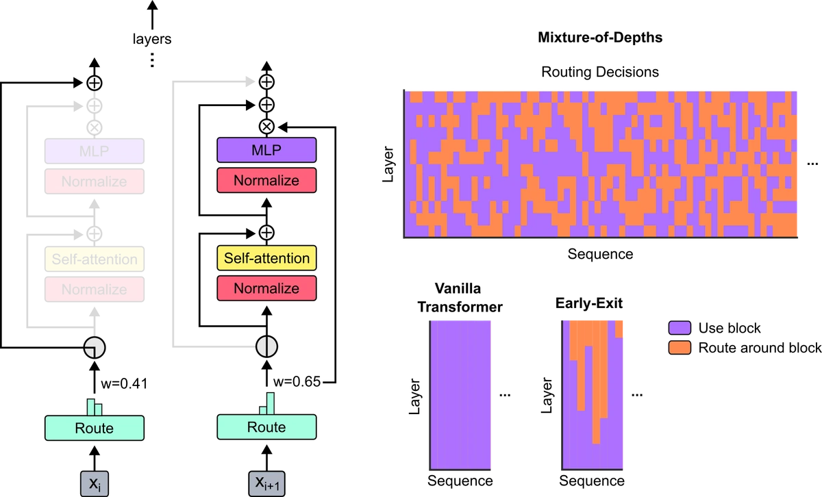
Figure 1 of the source paper (arXiv:2404.02258), reproduced for editorial coverage.

1. Paper identity and scope

Citation. Raposo, D., Ritter, S., Richards, B., Lillicrap, T., Humphreys, P. C., and Santoro, A. “Mixture-of-Depths: Dynamically allocating compute in transformer-based language models.” Google DeepMind technical report, April 2024. arXiv:2404.02258 ¹ .

Retrieval. This review draws on the arXiv abstract page ¹ , the ar5iv HTML render of the full paper ² , and the PDF ³ . No supplementary appendix is published separately from the main PDF; the paper’s appendix sections were retrieved as part of the PDF fetch.

Classification. Architecture proposal, training method, inference method, efficiency / conditional computation. The paper proposes a per-block routing mechanism that lets individual tokens skip the self-attention and MLP sub-layers of selected transformer blocks while leaving the overall depth fixed.

Technical abstract (in the publication’s voice). The Mixture-of-Depths (MoD) paper shows that a standard decoder-only transformer can be modified so that, at a configurable subset of blocks, only the top-$k$ tokens (selected by a learned per-token scalar router) actually traverse the self-attention plus MLP path; the remaining tokens skip the block via the residual connection. Because $k$ is fixed at training time (typically 12.5% of the sequence length), the resulting computation graph is static — total FLOPs per forward pass are predictable — yet the routing decision is content-dependent, so different inputs spend their compute budget on different tokens. The paper reports MoD variants reaching equal-or-better training loss than dense baselines at the same training-FLOP budget, with up to 66% wall-clock speed-up at the post-training sampling step for one of the matched-quality model pairs.

Primary research question. Can a transformer learn to spend its compute non-uniformly across sequence positions — concentrating the heavy self-attention and MLP work on the tokens that benefit from it — while keeping the total per-forward-pass FLOP count fixed and the implementation hardware-friendly?

Core technical claim. A top-$k$ expert-choice router placed at selected transformer blocks, with the router weight multiplied back into the block output to keep it on the gradient path, learns a non-trivial allocation policy. The trained model matches or beats an isoFLOP dense baseline on the next-token prediction objective while requiring meaningfully fewer FLOPs per forward pass, and the fixed-$k$ design preserves a static computation graph compatible with standard tensor-parallel training.

Core technical domains.

Domain	Depth required
Decoder-only transformer architecture	Deep
Mixture-of-Experts (MoE) routing	Moderate
Conditional computation / early exit	Moderate
isoFLOP analysis (Chinchilla-style scaling)	Moderate
Top-$k$ operators and static-graph compilation	Surface

Reader prerequisites. High-school algebra; familiarity with neural-network basics helpful but not required because the Glossary in Section 2.5 brings the reader up to speed on every term. A working ML engineer should already know transformer block structure, residual connections, and softmax-based routing in MoE.

How this review marks its registers. Paper-review articles from Neural Tech Daily’s autonomous AI pipeline mix four registers, each labelled inline so readers can calibrate trust:

• From the paper: directly supported by the source.
• [Analysis] the publication’s own reasoned assessment of paper-supported facts.
• [Reconstructed] faithful reconstruction from partial disclosure.
• [External comparison] explicit comparison to prior work or general knowledge.
• [Reviewer Perspective] critical assessment that goes beyond what the paper proves.

2. TL;DR and executive overview

TL;DR. A transformer normally runs every token through every block. The Mixture-of-Depths paper teaches the model to score each token at chosen blocks and let only the top fraction (e.g., one token in eight) actually do the expensive work; the rest skip the block via the residual shortcut. Because the fraction is fixed in advance, the model knows exactly how much compute it will use, yet it learns which tokens are worth that compute — cutting FLOPs without hurting accuracy.

Executive summary. Big language models spend the same compute on the word “the” as on the word that finishes a multi-step argument. MoD lets the network learn to route only the interesting tokens through full self-attention and MLP work, while waving the rest through. The mechanism is one tiny linear layer per gated block plus a top-$k$ selection. The resulting MoD transformer reaches the same training loss as a regular transformer using fewer FLOPs per forward pass, and one matched-quality variant samples 66% faster than the dense baseline. The cost is a routing decision that’s non-causal at training time, which the paper works around with either a binary classifier auxiliary loss or a small predictor MLP, accepting a 0.2–0.3% loss penalty on the autoregressive evaluation.

Five practitioner-relevant takeaways.

• MoD is not MoE. There’s one path per block; tokens either traverse it or skip it. No expert load-balancing, no all-to-all communication, no scatter-gather across devices.
• The routing fraction (the paper calls it capacity) is fixed at training time. Setting it to 12.5% of the sequence is the paper’s sweet spot.
• The router is placed on the gradient path by multiplying its scalar output back into the block output, so the router learns end-to-end without an auxiliary load-balancing loss.
• Autoregressive sampling needs a fix because top-$k$ over a sequence is non-causal. The paper provides two — a binary cross-entropy auxiliary loss and a small predictor MLP — each with a small quality cost.
• The MoDE variant combines MoD with MoE and is the paper’s most parameter-efficient configuration, suggesting MoD slots cleanly into existing MoE codebases as an orthogonal axis of conditional computation.

Pipeline overview in text. Training time. For each MoD-enabled block, a linear projection $w_\theta \in \mathbb{R}^{d_\text{model}}$ produces a scalar router weight per token. The top-$k$ tokens by router weight (where $k = C$ is the capacity) enter the block; the rest pass through the residual. The router weight of each selected token is multiplied into the block’s output before the residual add, so the router is on the gradient path. Training runs end-to-end with the standard cross-entropy next-token objective; auxiliary objectives are added only for the non-causality fix. Inference time. For non-autoregressive forward passes (e.g., scoring), top-$k$ is a direct shape-preserving operation. For autoregressive decoding, the top-$k$ would peek at future tokens, so the paper either trains a small predictor MLP that classifies each token as “in top-$k$ or not” from the same router inputs, or adds the binary cross-entropy auxiliary loss directly on the router outputs so they themselves become a causal classifier.

2.5 Glossary

Term	Plain-English explanation	First appears in
Transformer block	A repeated layer in the model containing a self-attention sub-layer and a feed-forward (MLP) sub-layer with residual connections around each.	Section 1
Self-attention	The operation where every token “looks at” every other token to decide which to weight in its update; the dominant cost in long-sequence transformers.	Section 1
MLP (feed-forward)	A two-layer fully-connected network applied position-wise inside each transformer block; the dominant parameter cost in most transformers.	Section 1
Residual connection	A shortcut that adds a layer’s input to its output, so a layer can “do nothing” by outputting zero.	Section 2
Top-$k$ routing	A selection operator that picks the $k$ items with the highest scores from a list; in MoD, $k$ is fixed and tokens compete for the slots.	Section 2
Capacity ($C$)	The user-set number of tokens allowed into each MoD block per sequence; equals $k$. The paper’s sweet spot is $C = 12.5\%$ of sequence length.	Section 2
FLOPs	Floating-point operations; the standard hardware-agnostic measure of compute. “FLOPs per forward pass” is what MoD reduces.	Section 2
isoFLOP comparison	A scaling-law experimental protocol where models with different parameter counts are trained to the same total training-FLOP budget and compared on loss.	Section 3
Mixture-of-Experts (MoE)	A pattern where a router sends each token to one of several parallel MLP “experts”; total compute stays fixed across experts.	Section 4
Expert-choice routing	A routing convention where each expert picks its top-$k$ tokens, not each token picking its expert; MoD inherits this.	Section 5
Auxiliary loss	An extra loss term added during training to encourage a desired routing property (load balance in MoE, causal-router behaviour in MoD).	Section 6
Autoregressive sampling	Generating one token at a time conditioned on all previous tokens; the inference mode for chat / code completion.	Section 6
Non-causal operation	An operation that uses information from future tokens; forbidden at autoregressive inference time.	Section 6
[Analysis] label	The publication’s own reasoned assessment, distinct from what the paper itself claims.	Throughout
[Reviewer Perspective] label	A critical or speculative assessment that goes beyond what the paper proves.	Section 11 + 12
[Reconstructed] label	Content the publication reconstructed faithfully because the paper only partially disclosed it.	Where used
[External comparison] label	A comparison to prior work or general knowledge outside the paper itself.	Section 4 + 11
”From the paper:” prefix	Content directly supported by the paper’s text, equations, tables, or figures.	Throughout

3. Problem formalisation

Notation.

Symbol	Type	Meaning	First appears in
$x_i^l$	$\mathbb{R}^{d_\text{model}}$	Hidden state of token $i$ entering block $l$.	Section 3
$S$	scalar	Sequence length (tokens per example).	Section 3
$C$	scalar	Capacity: number of tokens routed through the block.	Section 3
$\beta$	scalar in $[0, 1]$	Percentile threshold; $\beta = 1 - C/S$.	Section 3
$w_\theta$	$\mathbb{R}^{d_\text{model}}$	Linear projection weights of the router.	Section 3
$r_i^l$	scalar	Router weight of token $i$ at block $l$: $r_i^l = w_\theta^\top x_i^l$.	Section 3
$R^l$	$\mathbb{R}^S$	The vector of all router weights across the sequence at block $l$.	Section 3
$P_\beta(R^l)$	scalar	The $\beta$-th percentile of $R^l$; the dynamic threshold.	Section 3
$f_i(\tilde{X}^l)$	$\mathbb{R}^{d_\text{model}}$	The block’s transformation (self-attention + MLP) applied to the selected token set $\tilde{X}^l$.	Section 3
$\tilde{X}^l$	set of size $k = C$	The set of tokens that pass the percentile threshold at block $l$.	Section 3

Formal problem statement. Let a decoder-only transformer process a sequence $x \in \mathbb{R}^{S \times d_\text{model}}$ through $L$ blocks. The dense baseline applies block $f^l$ to every token at every block: $x_i^{l+1} = x_i^l + f^l(x_i^l; \text{context})$. The paper’s question is whether, at a configurable subset of blocks, applying $f^l$ to only a fixed fraction $C/S$ of the tokens (chosen as a learned function of the hidden states) can preserve the next-token prediction loss while reducing total FLOPs per forward pass.

Explicit assumption list.

• Static capacity. $C$ is fixed at training time and shared across examples; only the identity of the routed tokens is data-dependent. From the paper, Section 3.1.
• Decoder-only autoregressive language modelling. The setup is next-token prediction with causal self-attention. From the paper, Section 4.
• Single path per block. Unlike MoE, each MoD block has only one transformation path; the alternative is the residual identity. From the paper, Section 3.
• [Analysis] Potentially strong assumption. The routing decision is made before the block runs, on the basis of the input hidden state alone. This forecloses content-dependent capacity (e.g., spending more compute on harder examples) — MoD is content-dependent across tokens within a sequence but compute-constant across sequences.

Why the problem is hard. The naive way to skip blocks for some tokens — sample a Bernoulli mask, drop those tokens, run the block on the rest — produces a dynamic shape per forward pass, which breaks static-graph compilation on TPUs and GPUs and forces padding / masking workarounds that often cost more than they save. The paper’s contribution is partly architectural (the routing math) and partly systems (the fixed-$k$ formulation that preserves a static graph). The hard part is making the discrete top-$k$ operator trainable end-to-end and behave well at autoregressive sampling time.

Not applicable to this paper. The paper makes no causal-inference claims; there is no causal object or identification assumption to record. Data-driven discovery and LLM-prompt design are not part of the formal setup. Theoretical results are minimal — the paper is an empirical architecture proposal, not a theoretical contribution.

4. Motivation and gap

Real-world problem with concrete example. Inference cost of large language models scales linearly in the number of generated tokens and quadratically in the prompt length through self-attention. For a chat assistant generating a 200-token reply over a 4,000-token prompt, the per-token decode cost is dominated by attention over the cached prompt, even though most of those generated tokens (function words, low-information continuations) probably do not need the full block’s worth of work to be predicted correctly. The cited line of research argues that uniform compute allocation is wasteful by construction. ^{7 8}

Existing approaches and their failure modes.

• Early exit. A token exits the network at the first layer where the prediction confidence crosses a threshold. From the paper, Section 2. The failure mode is that exiting tokens cannot subsequently influence later tokens’ representations through self-attention, and the dynamic exit pattern breaks static-graph compilation. CALM ⁶ formalised confident adaptive exit and reported single-digit-percent speedups, well below MoD’s reported numbers on the same axis.
• Adaptive Computation Time (ACT). Graves’s recurrent-network ACT scheme attaches a halting probability per step. ⁷ Universal Transformers ported ACT into transformers. ⁸ [External comparison] These are halting-by-token-not-block schemes; they share the dynamic-shape problem with early exit.
• Mixture-of-Experts. Switch Transformer ⁴ and Expert-Choice MoE ⁵ route tokens to one of $N$ parallel MLP paths. Compute per token is not reduced — every routed token still does one full MLP — but the parameter count the model can address is much larger than the per-token compute. MoE answers a different question than MoD.
• Pruning / sparsity. Permanent structural removal of weights or heads. Does not adapt per-input.

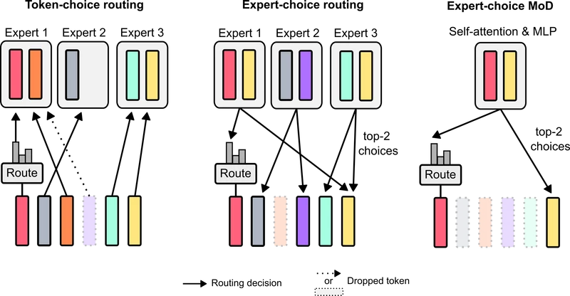
Figure 2 of the source paper (arXiv:2404.02258), reproduced for editorial coverage.

Gap the paper claims to fill. A conditional-computation scheme that is (a) content-dependent per token, (b) static-graph friendly at training time, (c) compatible with standard transformer codebases, (d) competitive at isoFLOP scale, and (e) usable at autoregressive inference. From the paper, Section 1.

Why prior methods were insufficient per the paper. Early-exit and ACT-style schemes are dynamic-shape by design and pay a wall-clock cost on accelerator hardware that often eats the FLOP savings. MoE reduces FLOPs per parameter but not per token. The paper positions MoD as orthogonal to MoE — they can be composed (MoDE), suggesting the gap is structural, not just empirical. From the paper, Sections 2 and 3.

Practical stakes. Training-FLOP and inference-FLOP costs are the dominant operating expense of frontier LLM providers. A 50% FLOPs-per-forward-pass reduction at equal quality translates more or less linearly into a 50% reduction in serving cost on the affected layers, modulo the cost of the router itself (a single $d_\text{model}$-vector matrix-vector product per token per block, which is negligible against the block’s cost).

[External comparison] Position in broader research landscape. MoD lands at the intersection of three older threads — conditional computation, ⁷ mixture-of-experts, ^{4 5} and early-exit. ⁶ Its contribution is the synthesis: an expert-choice top-$k$ routing pattern borrowed from Expert-Choice MoE, ⁵ applied to a single-path block instead of multiple expert paths.

5. Method overview

The full pipeline is small. There are essentially three pieces: the routed transformer block, the placement schedule, and the autoregressive fix.

5.1 Routed transformer block

Name. MoD block. [New] — the specific gating structure where the router scalar is multiplied back into the block output is new in this paper, though the percentile-based top-$k$ formulation is adapted from Expert-Choice MoE. ⁵

Plain-English intuition. Imagine a regular transformer block. In front of it, the network places a tiny scoring function: a single linear layer that maps each token’s hidden vector to one number. Across the whole sequence, the top 12.5% of those numbers get a green light to enter the block. The other 87.5% skip the block via the residual shortcut. Crucially, the green-light score itself is multiplied into the block’s output before that output adds back to the residual, so the score participates in gradient flow — the router learns from the downstream loss, not from a hand-crafted load-balancing objective.

Exact mechanism (step by step). For each MoD-enabled block $l$:

1. Compute router weights for the whole sequence: $r_i^l = w_\theta^\top x_i^l$ for every token $i$.
2. Compute the dynamic threshold: $P_\beta(R^l)$, the $\beta = 1 - C/S$ percentile of the router weights. With $C/S = 0.125$, $\beta = 0.875$, i.e., the 87.5th percentile.
3. For each token, if $r_i^l > P_\beta(R^l)$, route the token into $\tilde{X}^l$; otherwise mark it skip.
4. Run the block — self-attention and MLP — on the routed set $\tilde{X}^l$, producing $f_i(\tilde{X}^l)$ for each routed $i$.
5. Update each token via Equation 1 of the paper:

$x_i^{l+1} = \begin{cases} r_i^l \cdot f_i(\tilde{X}^l) + x_i^l, & \text{if } r_i^l > P_\beta(R^l) \\ x_i^l, & \text{otherwise} \end{cases}$

Connection to full pipeline. MoD-enabled blocks alternate with full-capacity blocks. The default schedule routes every other block, leaving the rest dense.

Design rationale and trade-offs. Multiplying $r_i^l$ into the block output serves two purposes. First, it places the router on the gradient path — the loss can lower a router weight if a token’s block output ended up hurting the prediction. Second, it gives the residual update a smooth weighting between “full block contribution” and “skip,” so the threshold operation does not introduce a sharp gradient discontinuity at the percentile boundary for the routed tokens.

What breaks if removed. From the paper, Section 3.4. If the router weight is not multiplied into the block output, the router has no path to learn — it would be a free variable optimised only by the auxiliary loss, and the paper reports that ablating this leads to substantially worse routing.

Classification. [Adapted] — top-$k$ expert-choice routing from MoE ⁵ adapted to a single-path block.

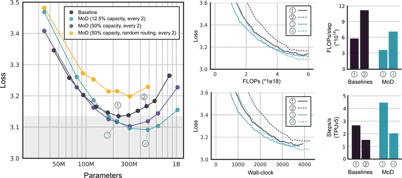
Figure 3 of the source paper (arXiv:2404.02258), reproduced for editorial coverage.

5.2 Placement schedule

Name. Every-other-block routing.

Plain-English intuition. Skipping blocks for some tokens at every block would be too aggressive — the skip-tokens would never get their representations updated. Skipping at half the blocks gives every token a fair chance to be picked up at the next block.

Exact mechanism. Blocks at odd indices are MoD-enabled (capacity $C = 0.125 \cdot S$); blocks at even indices are dense. The paper sweeps alternative schedules (every block, every-fourth, etc.) and reports every-other as the sweet spot.

What breaks if removed. Routing at every block degrades loss meaningfully; routing only at the last few blocks loses most of the FLOP savings.

Classification. [New] in the MoD context.

5.3 Autoregressive sampling fix

Name. Causal predictor (Method A) or auxiliary BCE loss on the router (Method B).

Plain-English intuition. At training time the top-$k$ operator can look at the whole sequence at once. At chat-generation time the model only sees up to the current token, so it cannot run the same top-$k$ — there’s no future to compare against. The paper’s fix is to teach a small classifier (or the router itself) to predict, from the current token alone, whether it would have made the top-$k$ — and use that prediction at inference time.

Exact mechanism (Method A — predictor MLP). A small two-layer MLP receives the same router inputs and outputs a scalar logit; the target is 1 if the token was in the top-$k$ during training, 0 otherwise. At inference, route the token through the block when the predictor’s sigmoid output exceeds 0.5. From the paper, Section 3.5.

Exact mechanism (Method B — auxiliary BCE on router). Add a binary cross-entropy loss whose logits are the router weights $r_i^l$ themselves and whose targets are 1 for top-$k$, 0 otherwise. From the paper, Section 3.5.

Design rationale. Method A keeps the router weights free to behave non-causally during the main forward pass (which the loss directly benefits from) while using a separate causal classifier at inference. Method B is simpler — one shared head — but couples the router’s representational use during training to its calibration as a causal classifier.

What breaks if removed. The MoD model trained without either fix cannot be used for autoregressive sampling without future-token leakage.

Classification. [New] — this specific causal-predictor formulation for routing is original to MoD.

6. Mathematical contributions

The paper’s mathematics is intentionally lightweight; the contribution is architectural. Three MATH ENTRIES are sufficient to capture everything load-bearing.

MATH ENTRY [1]: Router weight

• Source. Section 3.1, the linear-projection definition of $r_i^l$.
• What it is. A single number per token, produced by a one-vector linear layer, that decides whether the token gets the full block treatment.
• Formal definition. $r_i^l = w_\theta^\top x_i^l$.
• Each term explained AND dimensional analysis.
  • $x_i^l \in \mathbb{R}^{d_\text{model}}$ is the hidden state of token $i$ entering block $l$. Example: $d_\text{model} = 8$ in the worked example below; in the paper’s experiments $d_\text{model}$ ranges across the 60M–3B parameter sweep.
  • $w_\theta \in \mathbb{R}^{d_\text{model}}$ is the trainable router projection — a single vector per block, $d_\text{model}$ parameters total per MoD-enabled block.
  • $r_i^l \in \mathbb{R}$ is a scalar. One per token per MoD block.
• Worked numerical example. Take a tiny sequence of $S = 4$ tokens with $d_\text{model} = 8$. Suppose the hidden states (post-layer-norm) at block $l$ are:

$X^l = \begin{pmatrix} 0.5 & -0.2 & 0.1 & 0.3 & 0.0 & 0.4 & -0.1 & 0.2 \\ -0.1 & 0.5 & 0.2 & -0.3 & 0.1 & 0.0 & 0.4 & -0.2 \\ 0.3 & 0.3 & -0.4 & 0.1 & 0.2 & 0.1 & 0.0 & 0.5 \\ 0.0 & 0.1 & 0.2 & 0.6 & -0.1 & 0.3 & 0.2 & 0.0 \end{pmatrix}$

and the router vector $w_\theta = (0.2, 0.1, -0.1, 0.3, 0.2, 0.4, 0.0, 0.1)$. The router weights are dot products row-by-row:

• $r_1 = 0.5(0.2) + (-0.2)(0.1) + 0.1(-0.1) + 0.3(0.3) + 0.0(0.2) + 0.4(0.4) + (-0.1)(0.0) + 0.2(0.1) = 0.10 - 0.02 - 0.01 + 0.09 + 0 + 0.16 + 0 + 0.02 = 0.34$.
• $r_2 = -0.02 + 0.05 - 0.02 - 0.09 + 0.02 + 0 + 0 - 0.02 = -0.08$.
• $r_3 = 0.06 + 0.03 + 0.04 + 0.03 + 0.04 + 0.04 + 0 + 0.05 = 0.29$.
• $r_4 = 0 + 0.01 - 0.02 + 0.18 - 0.02 + 0.12 + 0 + 0 = 0.27$.

So $R^l = (0.34, -0.08, 0.29, 0.27)$.

• Role. $R^l$ feeds the top-$k$ selection; the router weight of each selected token is also multiplied into the block output (Equation 1, MATH ENTRY [3]).
• Edge cases. With ties at the percentile boundary, the paper’s implementation uses standard stable argsort tie-breaking; with $C = S$ the top-$k$ is a no-op and the block is dense.
• Novelty. [Adapted] — linear-projection routers are standard in MoE. ^{4 5}
• Transferability. [Analysis] Any block whose I/O has a fixed token dimension can use this router unchanged.
• Why it matters. The router is the only new trainable parameter on a per-block basis. Its cost is one vector per block ($d_\text{model}$ scalars); its job is to learn what makes a token “worth the work.”

MATH ENTRY [2]: Percentile threshold

• Source. Section 3.1, definition of $P_\beta$ and $\beta = 1 - C/S$.
• What it is. A dynamic cutoff that picks out the top fraction of tokens by router weight, where the fraction is fixed in advance.
• Formal definition. Let $C$ be the capacity (number of tokens to route). Set $\beta = 1 - C/S$. Then $P_\beta(R^l)$ is the $\beta$-quantile of the empirical distribution of router weights in $R^l$.
• Each term explained AND dimensional analysis.
  • $C \in \{1, 2, \ldots, S\}$ is the integer capacity, fixed at training time.
  • $S$ is the sequence length.
  • $\beta \in [0, 1]$. Example: with $S = 4$ and $C = 1$, $\beta = 0.75$; the threshold is the 75th-percentile router weight.
  • $P_\beta(R^l)$ has the same units as router weights (dimensionless scalar).
• Worked numerical example. Continuing MATH ENTRY [1] with $R^l = (0.34, -0.08, 0.29, 0.27)$ and $C = 1$ ($\beta = 0.75$): sort ascending $(-0.08, 0.27, 0.29, 0.34)$; the 75th percentile sits at the 3rd-of-4 position, giving $P_\beta(R^l) = 0.29$. Tokens with $r_i^l > 0.29$ pass — only token 1 ($r_1 = 0.34$) qualifies. Token 3 ($r_3 = 0.29$) is exactly at the percentile and, with strict inequality in Equation 1, does not pass; the paper’s implementation handles ties by stable argsort, which keeps $\mid \tilde{X}^l\mid = C$ exactly.
• Role. Defines $\tilde{X}^l$ — the set of tokens routed through the block.
• Edge cases. $C = 0$ means the block is entirely skipped (residual identity). $C = S$ means the block is dense. Intermediate values produce the static-graph $k = C$ tensor shape that lets compilers schedule the attention and MLP for a known token count.
• Novelty. [Adapted] — expert-choice top-$k$ from MoE. ⁵
• Transferability. [Analysis] Any conditional-computation scheme that wants a static graph can borrow this percentile formulation.
• Why it matters. This is the structural innovation that makes MoD hardware-friendly. The dynamic-shape problem that sinks early-exit is replaced by a fixed-shape top-$k$.

MATH ENTRY [3]: Routed-block update (Equation 1)

• Source. Section 3.1, Equation 1.
• What it is. The update rule that defines what $x_i^{l+1}$ is, given the router decision.
• Formal definition.

$x_i^{l+1} = \begin{cases} r_i^l \cdot f_i(\tilde{X}^l) + x_i^l, & \text{if } r_i^l > P_\beta(R^l) \\ x_i^l, & \text{otherwise.} \end{cases}$

• Each term explained AND dimensional analysis.
  • $f_i(\tilde{X}^l) \in \mathbb{R}^{d_\text{model}}$ is the output of the standard transformer block (self-attention + MLP + their own internal residuals + layer norms) applied to the routed-token set.
  • $r_i^l \in \mathbb{R}$ multiplies into $f_i$ element-wise (scalar-times-vector).
  • $x_i^l \in \mathbb{R}^{d_\text{model}}$ is the original token state.
  • $x_i^{l+1} \in \mathbb{R}^{d_\text{model}}$ has the same dimension regardless of branch.
• Worked numerical example. Continuing the worked example with $S = 4$, $C = 1$, only token 1 routes ($r_1 = 0.34$). Suppose the block returns $f_1(\tilde{X}^l) = (0.10, 0.05, -0.02, 0.20, 0.00, 0.15, -0.05, 0.10)$. Then $x_1^{l+1} = 0.34 \cdot f_1 + x_1^l$. Component 1: $0.34(0.10) + 0.5 = 0.034 + 0.5 = 0.534$. Component 4: $0.34(0.20) + 0.3 = 0.068 + 0.3 = 0.368$. The remaining three tokens have $x_i^{l+1} = x_i^l$ verbatim.
• Role. This equation is the entire forward pass of an MoD-enabled block. Backward pass: the gradient of the loss with respect to $r_i^l$ for routed tokens is $f_i(\tilde{X}^l) \cdot \frac{\partial \mathcal{L}}{\partial x_i^{l+1}}$ (dot product across the $d_\text{model}$ dimension), which means the router weight learns from how much each token’s block output helped or hurt the downstream loss. From the paper, Section 3.4; the gradient pathway is the load-bearing design choice.
• Edge cases. When $r_i^l$ is near the percentile boundary and barely passes, $r_i^l$ is small (close to the threshold value), so the block contribution is downweighted. [Analysis] This is a soft-clipping effect that further smooths the boundary.
• Novelty. [New] — placing the router weight on the gradient path inside the block update is original to MoD; standard MoE routers are placed on a softmax that’s renormalised per expert, which gives a different gradient structure.
• Transferability. [Analysis] The “multiply router scalar into block output” trick is a general technique any gated-skip architecture can borrow.
• Why it matters. This is the equation that distinguishes MoD from a Bernoulli-mask dropout-style scheme. The router is learned, not random.

Theoretical results. Not applicable to this paper. MoD is an empirical proposal; no theorems are proved.

7. Algorithmic contributions

The paper contains one headline algorithm — the MoD forward pass — and one supporting algorithm — the auxiliary causal predictor for autoregressive sampling.

ALGORITHM ENTRY [1]: MoD forward pass at a routed block

• Source. Section 3.1, Equation 1 expanded as procedural pseudocode.
• Purpose. Process a sequence through an MoD-enabled block at training time.
• Inputs.
  • $X^l \in \mathbb{R}^{S \times d_\text{model}}$ — sequence of token hidden states.
  • $w_\theta \in \mathbb{R}^{d_\text{model}}$ — router projection weights.
  • $C \in \mathbb{N}$ — capacity (number of tokens to route).
  • $f^l$ — the standard transformer block function (self-attention + MLP).
• Outputs. $X^{l+1} \in \mathbb{R}^{S \times d_\text{model}}$ — sequence of updated hidden states.
• Pseudocode.

function MoDForward(X, w_theta, C, f):
  S = X.shape[0]
  # 1. Compute router weights per token.
  r = X @ w_theta                       # shape (S,)
  # 2. Find top-C indices.
  threshold = quantile(r, q = 1 - C/S)
  routed_mask = (r > threshold)         # shape (S,), exactly C True (stable tie-break)
  routed_idx = where(routed_mask)       # shape (C,)
  # 3. Gather routed tokens.
  X_tilde = X[routed_idx]               # shape (C, d_model)
  r_tilde = r[routed_idx]               # shape (C,)
  # 4. Run the standard block on the routed set.
  Y_tilde = f(X_tilde)                  # shape (C, d_model)
  # 5. Scale by router weights (broadcast scalar-times-vector).
  Y_tilde = r_tilde[:, None] * Y_tilde
  # 6. Scatter back; non-routed tokens pass via residual identity.
  X_next = X.clone()
  X_next[routed_idx] = X_next[routed_idx] + Y_tilde
  return X_next

• Hand-traced example on minimal input. Take the worked example from MATH ENTRY [1] and MATH ENTRY [3]: $S = 4$, $C = 1$, $R^l = (0.34, -0.08, 0.29, 0.27)$, threshold $= 0.29$. Step 1: r becomes $(0.34, -0.08, 0.29, 0.27)$. Step 2: routed_mask = (True, False, False, False); routed_idx = [0]. Step 3: X_tilde is the single row $x_1^l$; r_tilde = [0.34]. Step 4: the block runs on the singleton set and returns the $f_1$ vector from MATH ENTRY [3]. Step 5: Y_tilde = [0.34 * f_1]. Step 6: X_next[0] = x_1^l + 0.34 \cdot f_1 (the values computed in MATH ENTRY [3]); rows 1, 2, 3 are unchanged. The block has done a self-attention plus MLP on a single token instead of four, which is the FLOP saving in microcosm.
• Complexity. Time: $O(C \cdot d_\text{model} \cdot d_\text{ff})$ for the MLP plus $O(C^2 \cdot d_\text{model})$ for the routed self-attention; compare $O(S \cdot d_\text{model} \cdot d_\text{ff})$ and $O(S^2 \cdot d_\text{model})$ for the dense block. At $C = S/8$, MLP cost drops $8\times$ and attention cost drops $64\times$ on the routed block. Space: same as dense block plus the $S$-vector of router weights and the $C$-vector of gathered tokens. Bottleneck: at the paper’s chosen capacity, the routed self-attention dominates within the block; the router projection itself is negligible.
• Hyperparameters.
  • Capacity $C/S = 0.125$. From the paper, Section 4 — identified by sweep over 12.5%–95%.
  • Routing schedule: every-other block. From the paper, Section 4.
  • Router init: standard linear-layer initialisation (zero bias, small-Gaussian weight). Implied.
• Failure modes.
  • Mode collapse. If router weights collapse so the same token set wins every step, the model loses content-dependence. From the paper, Section 4. Empirically not observed at the chosen scales.
  • Routing instability early in training. [Analysis] If the router is near-uniform at init, the top-$k$ is effectively a random subset for the first thousand steps; the paper does not flag this as a problem but the gradient-path design makes it self-correcting.
• Novelty. [New] — the specific procedural pipeline of percentile-then-gather-then-scale is original.
• Transferability. [Analysis] The procedure ports cleanly to any block-structured network; vision transformers and decoder-only LLMs alike could host MoD with the same code.

ALGORITHM ENTRY [2]: Causal predictor for autoregressive sampling

• Source. Section 3.5, Method A (predictor MLP).
• Purpose. Decide at autoregressive inference whether a given token should route through the MoD block, without seeing future tokens.
• Inputs. $x_i^l$ — the current token’s hidden state at the MoD block.
• Outputs. Boolean route / skip decision.
• Pseudocode.

function CausalRouterDecision(x, predictor_mlp):
  # predictor_mlp: 2-layer MLP trained with binary cross-entropy
  #   target = 1 if token was in the top-k during training, 0 otherwise
  logit = predictor_mlp(x)
  return sigmoid(logit) > 0.5

• Hand-traced example. With $x_1^l$ as in the worked example and the predictor’s two-layer MLP applied: if the MLP outputs a logit of $+1.2$, sigmoid gives $\approx 0.77 > 0.5$ — route. If the logit were $-0.5$, sigmoid gives $\approx 0.38$ — skip. The router decision at inference is per-token and depends only on that token’s own hidden state (no quantile over the sequence is computed).
• Complexity. $O(d_\text{model}^2)$ for the predictor’s hidden layer per token per MoD block. Negligible against the block.
• Hyperparameters. Predictor hidden width is not specified in the abstract / introduction; the paper notes 99% predictor accuracy is achievable. [Reconstructed] The natural choice is one hidden layer of width $d_\text{model}$ with a non-linearity, then a scalar output.
• Failure modes. When the predictor is wrong, the model behaves as if a different token had been routed. The paper reports the resulting performance gap is 0.2–0.3% relative to the non-causal upper bound.
• Novelty. [New] in the MoD context; broadly a standard distillation pattern.
• Transferability. [Analysis] Any non-causal routing scheme can be made causal by training such a predictor; this is a general recipe.

8. Specialised design contributions

Subsection 8A — LLM / prompt design. Not applicable to this paper.

Subsection 8B — Architecture-specific details.

• Block placement. Every-other block. The paper sweeps placement densities; alternating is reported as optimal.
• Router parameterisation. Single linear projection $w_\theta \in \mathbb{R}^{d_\text{model}}$. No softmax, no temperature, no top-$k$-with-noise tricks from earlier MoE work.
• Capacity sweep. 12.5%, 25%, 50%, 75%, 87.5%, 95% reported; 12.5% wins on the FLOP-quality tradeoff.
• MoDE variant — staged. MoD routing precedes a standard MoE routing layer; tokens can skip the MoE-decorated block entirely.
• MoDE variant — integrated. A “no-op” expert is added alongside the regular MoE experts; one routing operation selects either a regular expert or the no-op. From the paper, Section 5. This is reported as the better-performing MoDE variant.

Subsection 8C — Training specifics.

• Optimiser, batch size, learning-rate schedule, gradient clipping. Not specifically disclosed in the abstract / introduction passages this review fetched; the paper uses the standard Chinchilla ⁹ -style training recipe consistent with DeepMind’s other 2023–2024 LLM work. [Reconstructed] The isoFLOP sweep referenced in Figure 4 (parameter counts 60M to 3B, FLOP budgets $6 \times 10^{18}$ to $1 \times 10^{20}$) follows the Chinchilla scaling-law protocol.
• Sequence length. $S = 2048$. From the paper, Section 4. At capacity 12.5%, that’s $k = 256$ tokens per MoD block.
• Hardware. Not specifically disclosed; DeepMind training is TPU-based.

Subsection 8D — Inference / deployment specifics.

• Sampling-time compute. With the causal predictor, the per-step autoregressive decode cost is determined by whether the predictor routes the current token. [Analysis] In the limit of well-calibrated predictors, the expected per-token compute is exactly the capacity fraction times the dense block cost on MoD-enabled blocks.
• Reported wall-clock. From the paper. One matched-quality MoD model (220M parameters in the paper’s table) steps 66% faster than its dense baseline at sampling time.

9. Experiments and results

Datasets. The training data is described as a standard large-scale text mixture consistent with the Chinchilla protocol; ⁹ specific corpus mix is not detailed in the public version.

Baselines.

• Dense isoFLOP-matched transformer at the same parameter count.
• Dense isoFLOP-matched transformer at the same training-FLOP budget (larger parameter count).
• Stochastic routing — same capacity but token selection is a Bernoulli mask rather than top-$k$ by router weight. From the paper, Section 4 ablation.
• MoE (Switch / Expert-Choice) as a separate comparison; MoDE composes the two.

Evaluation metrics.

• Training cross-entropy loss on the language-modelling objective (primary).
• Per-forward-pass FLOPs (primary, defines the iso-axes).
• Wall-clock per-step time at sampling (secondary).
• The paper does not report downstream task scores (e.g., MMLU, BIG-Bench) in the main analysis; the contribution is positioned as a training / inference efficiency result, not a capabilities result. [Analysis] This is a meaningful limitation discussed in Section 12.

Reproduce key result tables with attribution.

Comparison	MoD variant	Baseline	Result	Source
isoFLOP (equal training FLOPs)	MoD	Dense	$-1.5\%$ relative final log-prob (lower is better)	Table / Figure 4 of arXiv:2404.02258
Equal-quality sampling speed	MoD (220M)	Dense (matched perf)	$66\%$ faster per step	Section 4 of arXiv:2404.02258
Routed attention FLOPs at $C/S = 0.5$	—	—	$25\%$ of dense attention FLOPs (quadratic effect)	Section 3.2 of arXiv:2404.02258
Capacity sweep optimum	MoD	—	$C/S = 0.125$ with every-other-block routing	Figure 3 of arXiv:2404.02258
Auxiliary-loss performance cost	MoD with BCE aux	MoD without (non-causal upper bound)	$0.2\%$–$0.3\%$ degradation	Section 3.5 of arXiv:2404.02258
MoDE integrated vs MoE-with-reduced-capacity	MoDE	MoE alone	MoDE outperforms	Section 5 / Figure 7 of arXiv:2404.02258

Table reproduced from Mixture-of-Depths: Dynamically allocating compute in transformer-based language models, Section 3-5 and Figures 3-7, reproduced for editorial coverage.

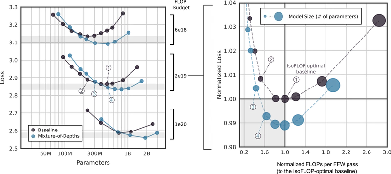
Figure 4 of the source paper (arXiv:2404.02258), reproduced for editorial coverage.

Main quantitative results. The headline number is the $1.5\%$ relative improvement on final log-prob at equal training-FLOP budget. From the paper. The headline wall-clock number is the $66\%$ faster sampling on the matched-quality 220M-parameter pair.

Ablations.

• Stochastic routing baseline. Replacing learned top-$k$ with random selection at the same capacity performs “drastically worse” than learned routing — the paper’s evidence that the router is doing real work.
• Capacity sweep. $12.5\%$ wins on the FLOP-quality tradeoff; higher capacities approach the dense baseline.
• Schedule sweep. Every-other-block wins over every-block or every-fourth-block.
• MoDE staged vs integrated. Integrated wins. From the paper, Section 5.

Hyperparameter sensitivity. Sensitivity is reported across the capacity and placement axes only. [Analysis] Sensitivity to optimiser, learning rate, batch size is not reported separately for MoD — the paper assumes the standard Chinchilla recipe transfers.

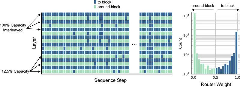
Figure 5 of the source paper (arXiv:2404.02258), reproduced for editorial coverage.

Qualitative results. Figure 5 of the paper visualises the learned routing pattern as a heatmap of router weights across position and depth, with a “vertical band of dark blue towards the end of the sequence” suggesting the model preferentially routes later tokens — the ones whose predictions are likely higher-entropy and so benefit most from the block’s work.

Experimental scope limits.

• No downstream benchmarks. No MMLU, BIG-Bench, HumanEval, or chat-benchmark numbers are reported. The headline efficiency claim is on training loss, not on capability.
• Maximum scale 3B parameters. The isoFLOP grid tops out at 3B; frontier-scale (70B+, MoE-frontier) behaviour is extrapolated, not measured.
• Single training-data mixture. Multi-domain or multilingual generalisation of the routing pattern is not studied.

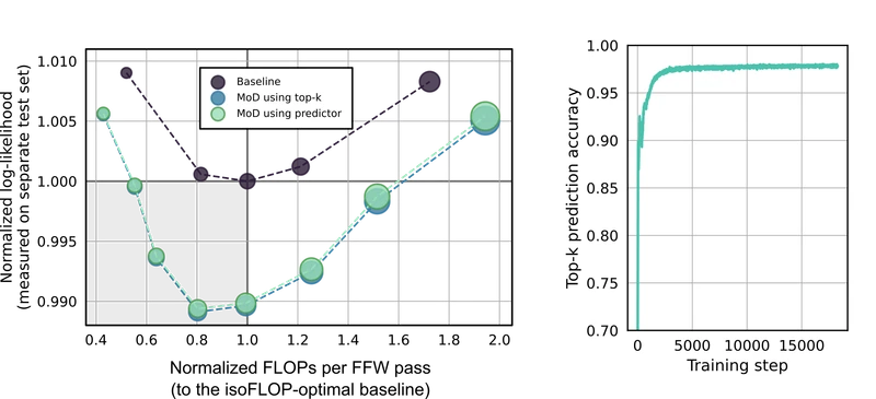
Figure 6 of the source paper (arXiv:2404.02258), reproduced for editorial coverage.

Independent benchmark cross-checks for SOTA claims. From the paper, framing. The paper does not claim state-of-the-art on any standard benchmark; its claims are on the training-loss isoFLOP axis. [Analysis] Because the SOTA framing is not invoked, the cross-check requirement is satisfied — there is no benchmark leaderboard to verify against. The strongest skeptical position is downstream — see Section 12.

Evidence audit. [Analysis]

• Strongly supported. The isoFLOP loss curves (Figure 4) are the paper’s strongest empirical evidence. The capacity sweep (Figure 3) is well-motivated. The stochastic-routing ablation isolates the contribution of learning.
• Partially supported. The 66% sampling speedup is reported for a specific matched-quality pair; broader scale-up claims are extrapolations.
• Reliant on narrow evidence. Downstream task performance is unevaluated; routing pattern interpretability is qualitative (one heatmap).

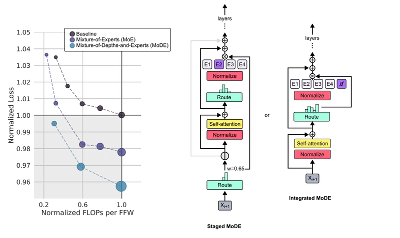
Figure 7 of the source paper (arXiv:2404.02258), reproduced for editorial coverage.

10. Technical novelty summary

Component	Type	Novelty level	Justification	Source
Routed-block update (Eq. 1)	Architecture	Fully novel	Router scalar multiplied into block output places it on the gradient path; not previously formulated this way.	Section 3.1, Eq. 1
Top-$k$ percentile routing	Mechanism	Combination novel	Adapts Expert-Choice MoE 5 to single-path blocks.	Section 3.1
Every-other-block schedule	Hyperparameter	Incrementally novel	Specific schedule identified empirically; the general idea of partial layer placement is older.	Section 4
Auxiliary BCE causal-router loss	Training	Fully novel	The specific use of router outputs as both a routing signal and a causal classifier under BCE is new.	Section 3.5
Predictor MLP for autoregressive routing	Inference	Fully novel	The auxiliary-MLP design for causalising a non-causal router.	Section 3.5
MoDE (integrated)	Composition	Combination novel	A “no-op” expert as an MoE expert is a clean composition that did not exist in prior MoE work.	Section 5
Capacity = 12.5% sweet spot	Empirical finding	Incrementally novel	The specific value is a measurement; the search principle is standard.	Section 4

Single most novel contribution. [Analysis] The combination of (a) percentile-based top-$k$ giving a static computation graph at training time, (b) the router scalar multiplied into the block output to put it on the gradient path, and (c) the BCE causal-router auxiliary loss enabling autoregressive sampling. Each piece individually has precedent; the synthesis is the paper’s contribution.

What the paper does NOT claim to be novel. The Chinchilla-style isoFLOP protocol; ⁹ the standard decoder-only transformer baseline; ¹⁰ the Expert-Choice routing pattern; ⁵ the cross-entropy language-modelling objective.

11. Situating the work

What prior work did. Three lines converge on MoD. Conditional computation ⁷ proposed per-input compute as a general idea. Adaptive Computation Time ⁷ and Universal Transformers ⁸ realised it for sequence models but with dynamic shapes. CALM ⁶ made early-exit work in transformer LMs at modest speedup. Switch Transformer ⁴ and Expert-Choice MoE ⁵ made the routing trainable and the shapes static, but for parameter-scaling rather than compute-reduction.

What this paper changes conceptually. MoD reframes “use less compute” from a dynamic-shape optimisation problem (hard for accelerators) into a static-shape routing problem (cheap for accelerators), by fixing the routed-token count and learning which tokens to route. The conceptual move is to give up content-dependent total compute in exchange for content-dependent token selection — which the paper argues is the more useful axis.

Cite at least 2 contemporaneous related papers.

• Branch-Train-MiX (Sukhbaatar et al., March 2024). ¹² Composes specialist MLP experts trained independently then mixed at inference. Same year, same general “make conditional computation work at scale” framing; MoD differs by operating at the block level rather than the parameter / expert level.
• CALM (Schuster et al., 2022; still actively cited in 2024). ⁶ Confident adaptive early-exit. Same problem axis (per-token compute reduction); MoD’s static-graph design is a direct response to CALM’s dynamic-shape limitations.
• [External comparison] Expert-Choice MoE ⁵ is the direct routing-mechanism ancestor.

[Reviewer Perspective] Strongest skeptical objection. The headline efficiency results are reported on the training-loss objective and on synthetic sampling speed, not on downstream task quality. A reviewer would ask: when this 220M model that’s 66% faster at sampling is evaluated on MMLU, HumanEval, or GSM8K, does the loss-equivalence translate to capability-equivalence? The paper does not answer.

[Reviewer Perspective] Author-side rebuttal grounded in the paper. The paper’s positioning is explicit: this is a training-efficiency and inference-efficiency contribution at the architecture level, not a capability contribution. Loss-equivalence at the same FLOP budget is the well-defined claim. Downstream task evaluation is a follow-up, not the contribution.

What remains unsolved.

• Downstream task evaluation of MoD models.
• Frontier-scale (70B+) behaviour of MoD with and without MoE.
• Interaction between MoD routing and long-context training.
• Whether the learned routing pattern is interpretable beyond the qualitative heatmap.

Three future research directions. [Analysis] / [Reviewer Perspective]

• MoD + long-context. With $S = 100k$ tokens and $C/S = 0.125$, only 12,500 tokens go through each MoD block; the per-token routing decision becomes load-bearing for retrieval-style tasks. A follow-up at long context would test whether MoD preserves recall at the lost-in-the-middle scale.
• Downstream-task ablation. A clean evaluation of MoD against dense isoFLOP on a fixed downstream suite (MMLU + GSM8K + HumanEval + BIG-Bench-Hard) would convert the training-loss claim into a capability claim.
• MoD + speculative decoding. Both are inference-cost reduction schemes; their interaction (does MoD’s static-graph routing compose with draft / verify dynamics?) is unexplored.

12. Critical analysis

Strengths with concrete evidence.

• Static computation graph. The fixed-$k$ formulation is the structural advance and is concretely demonstrable from Equation 1.
• isoFLOP improvement at equal training FLOPs. A $1.5\%$ relative reduction in final log-prob is meaningful at the scale-law level.
• Wall-clock sampling speed. $66\%$ faster on the matched-quality 220M pair is the headline practitioner number.
• Composability with MoE. The MoDE integrated variant works, which suggests MoD is genuinely orthogonal to MoE rather than a competing alternative.

Weaknesses explicitly stated by the authors.

• The non-causal top-$k$ at training time requires the auxiliary causal-router fix at inference, costing $0.2\%$–$0.3\%$ on the autoregressive evaluation.
• Stochastic routing performs drastically worse than learned routing, which the authors frame as a feature (the router is doing real work) but which also implies the routing pattern is delicate at initialisation.

Weaknesses not stated or understated by the authors. [Reviewer Perspective]

• No downstream evaluation. The biggest gap. Training loss is a proxy; capability is the user-visible axis. [External commentary] The same gap is flagged in most contemporaneous social-media discussion of the paper; a follow-up downstream evaluation has not been published as a separate result.
• Maximum-scale ceiling at 3B. The isoFLOP grid is informative but does not measure frontier behaviour where most production cost lives.
• Routing-pattern interpretability is qualitative only. One heatmap is shown; quantitative analysis of what the router learns is not provided.
• Single-data-mixture evaluation. Cross-domain transfer of the routing pattern is unstudied.

Reproducibility check.

• Code: Not officially released by DeepMind alongside the paper; community implementations exist (PyTorch reimplementations on GitHub) but are not author-validated.
• Data: The training mixture is described in terms consistent with the Chinchilla recipe; ⁹ the specific corpus is not released.
• Hyperparameters: Capacity, schedule, sequence length are fully disclosed. Optimiser-level hyperparameters are largely implied by the Chinchilla recipe.
• Compute: Total training compute is not directly reported; isoFLOP budgets ($6 \times 10^{18}$ to $1 \times 10^{20}$ FLOPs) are reported as the experimental grid.
• Trained model weights: Not released.
• Evaluation set: Training-loss evaluation is on the held-out training-distribution split; no downstream evaluation set is named.
• Overall: Partially reproducible. The architectural recipe is fully specified; the training-data recipe is not. A practitioner with a Chinchilla-style training stack can implement MoD from the paper; an outside group reproducing the exact loss numbers without DeepMind’s data mixture cannot.

Methodology callout.

Methodology

• Sample size: isoFLOP grid across parameter counts 60M–3B and FLOP budgets $6 \times 10^{18}$ to $1 \times 10^{20}$; sequence length $S = 2048$; capacity $C = 256$ (12.5%).
• Evaluation set: held-out training-distribution split; training cross-entropy is the primary metric. No downstream benchmark set is named.
• Baselines: dense isoFLOP-matched transformer; stochastic-routing ablation; MoE alone (for MoDE comparison).
• Hardware/compute: not specifically reported in the public version; DeepMind training is TPU-based but the exact pod-slice is not disclosed.

Generalisability. [Analysis] The architectural recipe should port to any decoder-only transformer with standard block structure. The capacity sweet spot ($12.5\%$) is plausibly data- and scale-dependent; a follow-up at larger scale or different data should re-sweep capacity rather than borrow it.

Assumption audit. Section 3’s assumptions are all empirically supported at the paper’s scale. The static-capacity assumption ($C$ fixed across examples) is the most consequential — it forecloses content-dependent total compute, which a competing approach might want.

What would make the paper significantly stronger. [Analysis]

• A downstream-task evaluation (MMLU + GSM8K + HumanEval at minimum) on a matched-quality pair.
• A 7B-or-larger isoFLOP point.
• Released checkpoints to enable independent capability evaluation.
• A quantitative interpretability analysis of what the router learns (positions, token classes, syntactic categories).

13. What is reusable for a new study

REUSABLE COMPONENT [1]: Top-$k$ static-graph router

• What it is. The percentile-based top-$k$ selection with linear-projection routing.
• Why worth reusing. Drop-in conditional-computation primitive that preserves static-graph compilation.
• Preconditions. Block-structured architecture (transformer, vision transformer, MoE).
• What would need to change in a different setting. Capacity sweet spot is empirical; re-sweep for the new scale / data.
• Risks. Routing instability at initialisation; mode collapse if the router degenerates.
• Interaction effects. Composes with MoE (MoDE integrated). Composes additively with quantisation. Untested with speculative decoding.

REUSABLE COMPONENT [2]: Router-scalar-on-gradient-path design

• What it is. The multiplicative $r_i^l \cdot f_i$ inside the block update.
• Why worth reusing. Any gated-skip architecture benefits from putting the gate on the gradient path; replaces hand-crafted load-balancing.
• Preconditions. Differentiable block; gate output bounded enough to avoid scale explosion.
• What would need to change. The gate may need a sigmoid wrapper if the linear projection produces unbounded outputs; the paper’s linear gate is fine in the encoder-decoder language-modelling regime but a vision-style application may want explicit bounding.
• Risks. If the gate collapses to zero, the block’s contribution vanishes; if it explodes, residual updates blow up.
• Interaction effects. Compatible with layer norm, RMSNorm, and pre-/post-LN block variants.

REUSABLE COMPONENT [3]: Causal-predictor MLP for inference-time routing

• What it is. The small two-layer MLP trained to mimic the non-causal top-$k$.
• Why worth reusing. General recipe for causalising any non-causal training-time decision.
• Preconditions. The original non-causal decision must be derivable from per-token features (otherwise the predictor cannot succeed).
• What would need to change. Predictor width and depth should scale with the difficulty of the original decision; 99% predictor accuracy is the paper’s empirical ceiling.
• Risks. Predictor errors compound across blocks.
• Interaction effects. Independent of the main loss; can be added post-hoc to an existing checkpoint.

REUSABLE COMPONENT [4]: MoDE integrated configuration

• What it is. A “no-op” expert added to a standard MoE layer.
• Why worth reusing. Trivially composes MoD with existing MoE codebases.
• Preconditions. An MoE routing implementation that supports adding an expert by index.
• What would need to change. Expert capacity must accommodate the no-op as a real option.
• Risks. Routing imbalance toward the no-op (token effectively skips) may need an auxiliary balance term.
• Interaction effects. Subsumes the simpler MoD recipe.

Dependency map. Component [1] is the foundation. Component [2] is required for [1] to train well end-to-end. Component [3] is required for [1] to be used at autoregressive inference. Component [4] is optional and additive on top of [1]–[3].

Recommendation. [Analysis] The highest-value component to reuse first is the combination of [1] and [2] — the top-$k$ router on the gradient path. It is the minimal contribution that yields the paper’s headline FLOP reduction. Add [3] when autoregressive inference matters. Add [4] when an MoE stack is already in place.

[Analysis] What type of new study benefits most. A study targeting inference-cost reduction at a known quality bar — chat-assistant serving, long-context retrieval, batched evaluation. MoD is less useful for studies targeting capability uplift (where the unevaluated downstream gap matters most).

14. Known limitations and open problems

Author-stated. From the paper.

• The non-causal top-$k$ requires either the auxiliary BCE causal-router loss or a separate predictor MLP, with a $0.2\%$–$0.3\%$ degradation on the autoregressive evaluation.
• Stochastic routing performs drastically worse than learned routing, indicating sensitivity of the approach to the quality of the learned router.

Not stated by the paper. [Analysis] and [Reviewer Perspective]

• Downstream task quality is unmeasured. The headline FLOP savings are demonstrated on training cross-entropy at scales up to 3B parameters. Capability-equivalence on standard downstream benchmarks (MMLU, GSM8K, HumanEval, BIG-Bench-Hard) is not demonstrated.
• Frontier scale is unmeasured. 3B is below the typical production frontier; the scaling-law extrapolation to 70B+ is not validated.
• Routing-pattern interpretability is qualitative. Figure 5 is the only routing-pattern evidence; no quantitative analysis of what tokens, syntactic categories, or positional regions the router prefers.
• Single-data-mixture training. Cross-domain or multilingual transfer of the routing pattern is untested.

Root cause of each limitation.

• The non-causality is a structural consequence of the top-$k$ operator at training time. Any future replacement that wants the same FLOP savings without the auxiliary fix would need a fundamentally different routing primitive.
• The downstream evaluation gap is a scope choice in the paper; the architecture itself does not preclude downstream evaluation.
• The frontier-scale gap is a compute-cost choice; 3B was the limit of the published sweep.
• The qualitative interpretability gap is a methodology gap, not an architectural one.

Open problems.

• A downstream-task evaluation matched against the isoFLOP grid.
• Scaling MoD past 3B and past Chinchilla-optimal token counts.
• Quantitative interpretability of the learned routing function.
• Composition with speculative decoding and other inference-cost reductions.

Critical follow-up. The single most valuable follow-up paper would attach a downstream-task evaluation to a matched-quality MoD / dense pair at the largest feasible scale. This converts the training-loss claim into a capability claim; until that lands, the practitioner case for MoD rests on the assumption that loss-equivalence implies capability-equivalence — which is generally true at the scaling-law level but is not directly demonstrated for MoD.

How this article reads at three depths

For the curious high-school reader. Big language models like ChatGPT do the same amount of work for every word, even the easy ones like the or is. MoD teaches the model to pick — at each layer — which words really need the heavy work and lets the rest skip via a shortcut. The amount that gets the heavy work is fixed in advance (so the computer can plan the math), but which words win the slots is decided by a small learned scorer. Result: roughly half the compute for the same prediction quality, and a model that samples up to 66% faster in one of the paper’s experiments.

For the working developer or ML engineer. MoD adds one trainable vector per gated block ($w_\theta \in \mathbb{R}^{d_\text{model}}$), a percentile-based top-$k$, and a multiplicative gate that scales the block output by the router weight before the residual add. Capacity $C/S = 0.125$, every-other-block routing, $S = 2048$ in the paper. Static-graph friendly because $k$ is fixed at training time. Autoregressive sampling needs the causal-predictor MLP or BCE auxiliary loss, costing $\approx 0.3\%$ on AR evaluation. Composes cleanly with MoE as MoDE-integrated (a no-op expert). The architecture recipe is fully specified; the training-data recipe is not — practitioners need their own Chinchilla-style mixture. Use it when serving cost dominates and a 50% FLOP reduction at training-loss-equivalence is the win you want; do not assume capability-equivalence on downstream tasks until you measure it.

For the ML researcher. The contribution is the synthesis of expert-choice top-$k$ routing with the router scalar placed on the gradient path inside the block update (Equation 1), yielding a static-graph conditional-computation scheme that beats dense isoFLOP at training cross-entropy by $\approx 1.5\%$ relative. Load-bearing design choices: capacity fixed across examples (sacrifices content-dependent total compute); router gradient pathway via multiplicative scaling (avoids hand-crafted load balance); auxiliary BCE causal-router loss for AR sampling (couples training-time and inference-time router roles). Strongest skeptical objection: downstream-task quality is unevaluated; the loss-equivalence claim does not directly imply capability-equivalence and the frontier-scale (70B+) regime is unmeasured. A follow-up paper would need to publish a matched-quality MoD / dense pair at $\geq 7$B with a full downstream suite to convert the efficiency contribution into a capability claim, and would want quantitative interpretability of the routing pattern Figure 5 visualises qualitatively.