The Llama 3 and Llama 4 technical reports — a multi-paper review

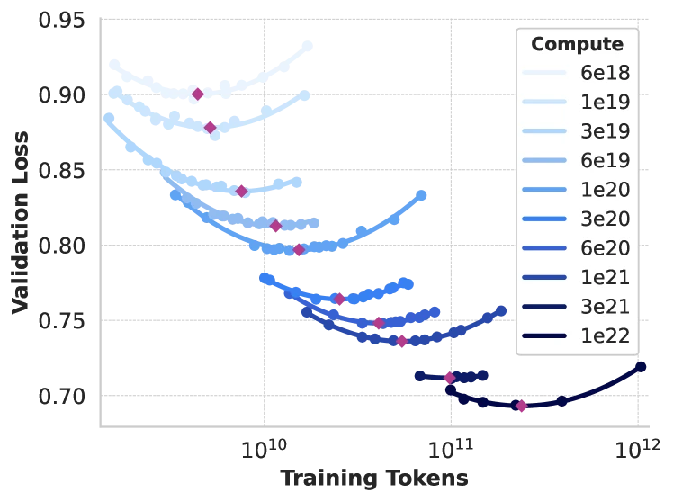
Figure 2 of The Llama 3 Herd of Models (arXiv:2407.21783), reproduced for editorial coverage.

1. Umbrella scope and paper identity

Citations.

• Grattafiori et al. and the Meta Llama team, “The Llama 3 Herd of Models,” arXiv:2407.21783, July 2024 ¹ . The flagship technical report covering Llama 3.0, 3.1, and 3.2 dense models from 8B to 405B parameters.
• Meta AI, “The Llama 4 herd: the beginning of a new era of natively multimodal AI innovation,” blog post, April 2025 ³ , accompanied by per-model cards on Hugging Face for Scout ⁴ and Maverick ⁵ . The Llama 4 release did not ship a single consolidated arXiv technical report at launch; the blog plus the model cards are the most authoritative public artefacts. This article treats them as the canonical source while flagging the disclosure-density gap relative to the Llama 3 paper.

Retrieval. The Llama 3 paper was retrieved in full via the ar5iv HTML render ² . The Llama 4 material was retrieved from Meta’s official AI blog ³ plus the Hugging Face model cards ^{4 5} . [Reconstructed] Several Llama 4 specifications surfaced in this article (active-parameter routing depth, expert capacity factor, exact training token count for Behemoth) are not disclosed in the public Meta material and have been left explicitly hedged where they appear.

Classification. Architecture proposal (Llama 4’s mixture-of-experts shift), training method (post-training pipeline across both releases), benchmark, application. Both releases are LLM-based; Llama 4 adds native multimodality via early-fusion vision tokens.

Technical abstract in the publication’s voice. The Llama 3 paper documents Meta’s transition from a 70B-class dense Transformer to a 405B-class one trained on roughly 15.6 trillion tokens at $3.8 \times 10^{25}$ floating-point operations, the largest publicly-documented dense-Transformer pretraining run as of mid-2024. The paper is unusually transparent: it discloses the scaling-law fitting procedure, the data mixture by category, the post-training cocktail of supervised fine-tuning plus rejection sampling plus six rounds of Direct Preference Optimization, the 4D parallelism layout across 16,000 H100 GPUs, and the hardware-failure statistics over a 54-day training window. The Llama 4 release in April 2025 then makes two architectural breaks from Llama 3: dense Transformers give way to sparse mixture-of-experts (MoE) routing, and vision is integrated via early fusion rather than the bolted-on compositional encoder used in Llama 3.2. The Llama 4 lineup at release is Scout (17B active, 109B total, 16 experts), Maverick (17B active, 400B total, 128 experts), and Behemoth (288B active, ~2T total, still training at announcement).

Primary research questions.

• Llama 3: How far can a dense Transformer scale with rigorous compute-optimal data scaling, and what post-training recipe produces a usable assistant from that base?
• Llama 4: Can an MoE design at fixed active-parameter budget match or beat the largest dense models on standard benchmarks while remaining serveable on a single H100 host?

Core technical claims.

• Llama 3: The Chinchilla-style power law $N^{*}(C) = 0.29 \cdot C^{0.53}$ fits Meta’s isoFLOP experiments across compute budgets from $6 \times 10^{18}$ to $10^{22}$ FLOPs and extrapolates to a compute-optimal 402B-parameter model trained on 16.55T tokens at the project’s $3.8 \times 10^{25}$ FLOP budget ^{1 2} .
• Llama 4: Scout’s 17B active parameters with 16 experts delivers 10M-token context via interleaved RoPE and inference-time attention temperature scaling; Maverick beats GPT-4o and Gemini 2.0 Flash on Meta’s evaluation suite while running on a single H100 DGX node ³ . [Analysis] The benchmark claim is the authors’ framing on their chosen evaluation harness; independent reproduction was contested at launch (see Section 11).

Core technical domains.

Domain	Depth
Transformer pretraining at frontier scale	Deep
Chinchilla scaling laws	Deep
Mixture-of-experts routing	Moderate
RLHF and DPO post-training	Deep
4D parallelism (TP / CP / PP / FSDP)	Moderate
Multimodal early fusion vs. compositional encoder	Moderate
Long-context training (RoPE, iRoPE)	Moderate

Reader prerequisites. Decoder-only Transformer basics, supervised fine-tuning, the rough shape of RLHF (SFT then reward model then preference optimisation). The Glossary in Section 2.5 brings the high-school reader up to speed on every other term.

Register labels used throughout. “From the paper:” prefix for paper-supported claims. [Analysis] for the publication’s own assessment. [Reconstructed] for content reconstructed from partial disclosure (heavily used for Llama 4 since the release lacks a formal technical report). [External comparison] for comparisons to prior or contemporaneous work. [Reviewer Perspective] for skeptical commentary beyond what the paper proves.

2. TL;DR and executive overview

TL;DR. Llama 3 is Meta’s last dense Transformer family, scaling from 8 billion to 405 billion parameters trained on roughly 15 trillion tokens of text using rigorous Chinchilla-style scaling laws to pick the model size. Llama 4 then switches to a sparse mixture-of-experts design where only a fraction of the network activates per token, letting the 400-billion-parameter Maverick model run on a single high-end server. Together the two releases document the practical recipe for training frontier-scale open-weights language models in 2024 and 2025.

Executive summary. The Llama 3 paper is the most detailed public account of a frontier dense-Transformer pretraining run yet published, covering scaling-law derivation, data mixture, six rounds of iterative DPO post-training, and 4D parallelism on 16,000 H100 GPUs. Llama 4, released eight months later, makes two structural breaks: dense Transformers give way to mixture-of-experts routing where a token activates 17 billion of up to 400 billion parameters, and vision becomes native via early-fusion tokens rather than a bolted-on encoder. The Llama 4 release was contested on launch over evaluation-harness choices; the Llama 3 paper’s level of disclosure was not matched. Together the two releases trace Meta’s bet on sparse activation as the path to keeping serving cost flat while total parameter counts climb.

Five practitioner-relevant takeaways.

1. The Llama 3 405B serving footprint is roughly an order of magnitude bigger than Maverick’s, even though Maverick has nearly the same total parameter count, because Maverick activates only 17B of those parameters per token. The MoE shift is fundamentally a serving-cost optimisation, not a quality optimisation.
2. For teams building on Llama 3 weights, the post-training recipe (SFT then rejection sampling then six rounds of DPO with NLL regularisation and $\beta = 0.1$) is the most rigorously documented public recipe and transfers directly to other base models.
3. Llama 4 Scout’s claimed 10-million-token context window relies on iRoPE (interleaved attention layers without positional encoding mixed with RoPE layers) and inference-time temperature scaling. Treat the 10M number as a stress-test capability, not a quality guarantee at full context.
4. The Llama 3 paper’s hardware-failure log (466 interruptions over 54 days, 78% of unexpected interruptions hardware-related, 58.7% of all unexpected issues from GPUs) is itself a contribution: anyone budgeting frontier-scale training should plan for it.
5. [Analysis] Meta’s compositional vision encoder in Llama 3.2 was a stopgap; Llama 4’s early-fusion approach is the architectural commitment. Teams choosing a multimodal open-weights base should default to Llama 4 family over Llama 3.2 for new builds.

Pipeline overview. Pretraining for both releases starts from raw web data plus code plus math plus multilingual sources, runs Chinchilla-style scaling-law experiments at small scale to pick the compute-optimal model and dataset size, then trains at the chosen point. Llama 3 is dense throughout; Llama 4 introduces MoE layers alternating with dense ones. Post-training in both runs SFT then rejection-sampling-then-DPO in Llama 3, with Llama 4 reportedly swapping the middle stage for “online RL” before a final “lightweight DPO” ³ . Inference for Llama 3 is straightforward auto-regressive decoding; Llama 4 adds top-k expert routing per token.

2.5. Glossary

Term	Plain-English explanation	First appears in
Transformer	The neural network architecture all modern large language models use; processes input as a sequence of tokens and predicts the next one.	Section 1
Token	The smallest unit of text the model sees; usually a sub-word piece like “ing” or “the”. Llama 3 has a 128,000-token vocabulary.	Section 1
Pretraining	The initial phase where the model learns from trillions of tokens of raw text by predicting the next word; produces the “base model”.	Section 1
Dense Transformer	A Transformer where every parameter participates in every forward pass; contrasted with sparse / MoE designs.	Section 1
Mixture of experts (MoE)	A design where the network has many “expert” subnetworks but a routing layer activates only a few per token; total parameter count is large while active parameters per token stay small.	Section 1
Active parameters	The number of parameters actually computed for a given token in an MoE model. Llama 4 Maverick has 17B active out of 400B total.	Section 1
Scaling law	An empirical formula relating model loss to model size and training tokens; used to pick the compute-optimal model for a given compute budget.	Section 1
Chinchilla scaling	DeepMind’s 2022 finding that model size and training tokens should grow together roughly equally with compute; used to size Llama 3.	Section 1
FLOP	”Floating-point operation”; the standard unit of compute for training. Llama 3 405B used $3.8 \times 10^{25}$ FLOPs.	Section 1
SFT (supervised fine-tuning)	Training the base model on curated high-quality (prompt, response) examples to learn the assistant format.	Section 2
DPO (Direct Preference Optimization)	A 2023 alignment method that replaces PPO-based RLHF with a single supervised loss over preference pairs. Llama 3 uses 6 rounds of it.	Section 2
Rejection sampling	Generating $K$ candidate responses per prompt and keeping only those scored highly by a reward model; used as the SFT-data filter in Llama 3 post-training.	Section 2
RoPE (Rotary Position Embedding)	A method for encoding token positions by rotating attention vectors; used in Llama 3 with a frequency base of 500,000 to support long contexts.	Section 5
iRoPE	Llama 4’s “interleaved RoPE”: alternating layers, some with RoPE positional encoding and some without; reportedly extends context to 10 million tokens.	Section 5
GQA (Grouped Query Attention)	An attention variant where multiple query heads share a single key/value head, reducing KV-cache memory; Llama 3 uses 8 KV groups across all sizes.	Section 5
4D parallelism	Splitting training across GPUs along four axes: tensor, context, pipeline, and data. Llama 3 uses all four to scale to 16,000 H100s.	Section 7
Early fusion (multimodal)	Treating image patches as just more tokens fed into the same Transformer as text, rather than running them through a separate encoder.	Section 8
[From the paper] prefix	Content directly supported by the cited paper or vendor disclosure.	Throughout
[Analysis] label	The publication’s own reasoned assessment, distinct from what the paper claims.	Throughout
[Reconstructed] label	Content reconstructed from partial disclosure where the source does not fully specify the detail; flagged so the reader can calibrate trust.	Section 1
[External comparison] label	A comparison to prior or contemporaneous work outside the paper itself (Chinchilla, Mixtral, DeepSeek-V3).	Section 4
[Reviewer Perspective] label	A skeptical or speculative assessment beyond what the source proves; surfaces independent commentary.	Section 11

3. Problem formalisation

Notation table.

Symbol	Type	Meaning	First appears in
$N$	Scalar	Model parameter count	Section 3
$D$	Scalar	Training token count	Section 3
$C$	Scalar	Training compute in FLOPs	Section 3
$L(N, D)$	Function	Cross-entropy loss as a function of model size and tokens	Section 3
$N^{*}(C)$	Function	Compute-optimal model size at budget $C$	Section 3
$\alpha$	Scalar	Scaling-law exponent (Llama 3 fits $\alpha = 0.53$)	Section 3
$A$	Scalar	Scaling-law prefactor (Llama 3 fits $A = 0.29$)	Section 3
$E$	Scalar	Total number of experts in MoE layer	Section 5
$k$	Scalar	Number of experts activated per token (top-$k$ routing)	Section 5
$G(x)$	Vector	Gating distribution over $E$ experts for token $x$	Section 5
$\pi_{\theta}$	Function	The trainable policy (language model)	Section 6
$\pi_{\text{ref}}$	Function	The frozen reference policy (typically the SFT model)	Section 6
$\beta$	Scalar	DPO temperature-like parameter; Llama 3 uses $\beta = 0.1$	Section 6

Formal problem statement. The pretraining problem is to find parameters $\theta$ that minimise the next-token cross-entropy loss

$\mathcal{L}_{\text{pre}}(\theta) = -\mathbb{E}_{x \sim \mathcal{D}_{\text{pre}}} \left[ \sum_{t=1}^{T} \log p_{\theta}(x_t \mid x_{<t}) \right]$

over a pretraining distribution $\mathcal{D}_{\text{pre}}$ of mixed web, code, math, and multilingual text, subject to a fixed compute budget $C$ measured in floating-point operations. The Chinchilla framing ⁶ then converts this into a joint optimisation over model size $N$ and training tokens $D$ where $C \approx 6 N D$ holds approximately for dense Transformers. The scaling-law experiments fit $N^{*}(C)$ and $D^{*}(C)$ empirically.

Explicit assumption list.

• Llama 3: The dense-Transformer compute formula $C \approx 6 N D$ holds across the fitting range $6 \times 10^{18}$ to $10^{22}$ FLOPs ² . [Analysis] Potentially strong assumption when extrapolating five orders of magnitude further to $3.8 \times 10^{25}$ FLOPs; the paper’s downstream-task fit is what validates the extrapolation, not the loss curve alone.
• Llama 3: The 15.6T-token training corpus is approximately deduplicated and quality-filtered such that token count is a meaningful measure of “training data seen” ² .
• Llama 4: The MoE compute formula adapts to active-parameter count $N_a$ rather than total $N_t$, with $C \approx 6 N_a D$ ³ . [Reconstructed] This is the standard MoE accounting convention; Meta does not state it explicitly in the blog post.
• Both: Quality of cross-entropy loss as a proxy for downstream-task quality at frontier scale.

Why the problem is hard. Three independent reasons. First, the search over $(N, D)$ pairs at the actual target compute is infeasible (one run at $3.8 \times 10^{25}$ FLOPs costs tens of millions of dollars); the scaling-law fit at smaller compute is the only practical method. Second, data quality matters more than data quantity at the upper end of the curve, and quality is not a single scalar; it interacts with filtering, deduplication, and mixture ratios in ways that small-scale experiments don’t fully predict. Third, at 16,000-GPU scale, hardware-failure rates make any single training run a distributed-systems engineering problem, not just an ML problem.

Data-driven setup. Llama 3’s pretraining data is, per the paper, approximately 50% general knowledge (web text), 25% mathematical and reasoning, 17% code, and 8% multilingual ² . The paper does not publish the underlying source URLs or dataset hashes. [Analysis] This is a notable disclosure gap relative to community open-data efforts like Dolma and FineWeb-Edu, and one of the reasons Llama-family models, while open-weights, are not open-data.

LLM-based role. Both releases are language models; in Llama 4 the LLM additionally serves as the multimodal backbone with vision patches projected directly into the token embedding space.

4. Motivation and gap

The real-world problem is that the highest-quality publicly-downloadable language models in 2023 (Llama 2 70B, Mixtral 8x7B ¹⁴ ) trailed the best closed models (GPT-4, Claude 2, Gemini 1.0) by a sizeable margin on the reasoning, code, and math benchmarks practitioners cared about. Meta’s stated motivation for Llama 3 is closing that gap with open weights; the 405B-parameter dense Transformer is the largest commitment of a single company to publishing a frontier-class open-weights base model.

Existing approaches and their failure modes per Meta’s framing ² :

• Llama 2 (70B): Trained on 1.8T tokens, significantly under-scaled relative to Chinchilla-optimal token counts. The paper explicitly cites this under-training as a gap Llama 3 closes by going to 15T+ tokens.
• GPT-4 / Claude / Gemini: Closed weights; the recipe was not reproducible. [External comparison] Independent estimates (e.g., from EpochAI, SemiAnalysis) place GPT-4 in the $\sim 10^{25}$ FLOPs regime, within the same compute order as Llama 3 405B.
• Mixtral 8x7B: Sparse MoE, but with 47B total parameters and routing only across feed-forward layers; significantly smaller than what Llama 4 later commits to.

The gap Llama 3 claims to fill is a fully-documented Chinchilla-optimal frontier-scale training run with permissive weights release. The gap Llama 4 claims to fill is an open-weights MoE family that matches or exceeds dense competitors at lower serving cost.

[External comparison] Position in the broader landscape: Llama 3 lands between DeepMind’s Chinchilla scaling work ⁶ on the theoretical side and Mistral’s MoE work ¹⁴ on the architectural side. Llama 4’s MoE shift comes after DeepSeek-V3 ¹³ demonstrated that a 671B-total / 37B-active MoE could match Llama 3 405B at significantly lower training cost (~$5.6M reported), which [Reviewer Perspective] is the unstated competitive context for Meta’s MoE pivot.

5. Method overview

5.1 Llama 3 architecture

[From the paper] ² Llama 3 is a dense, decoder-only Transformer with Grouped Query Attention (GQA) ¹⁰ , SwiGLU activations, RMSNorm pre-normalisation, and Rotary Position Embedding (RoPE) ¹¹ with a base frequency of 500,000. The 405B configuration uses 126 layers, hidden dimension 16,384, 128 attention heads, and 8 KV heads (16:1 query-to-KV ratio). The 8B and 70B variants share the same architectural choices at smaller scale. The tokenizer is 128,000 entries combining 100K from tiktoken plus 28K additional tokens for non-English coverage.

Plain-English intuition. A dense Transformer means every parameter is involved in every prediction. Llama 3 is “just bigger” relative to Llama 2: more layers, wider hidden dimension, more attention heads, and a longer context window after staged extension training. The architectural choices are deliberately conservative; the paper’s contribution is the scale and the rigour of the scaling-law derivation, not architectural novelty.

Design rationale. GQA shrinks the key-value cache memory at inference time by 16x for the 405B configuration; this is what makes serving 405B at 128K context feasible at all. RoPE base 500,000 was chosen to support long context up to 32,768 tokens stable, then extended via continued pretraining to 128K in six stages.

Classification. [Adopted] for the core architectural choices (GQA, RoPE, RMSNorm, SwiGLU all predate Llama 3); [Adapted] for the long-context extension recipe; [New] for the specific configuration and scaling-law fit.

5.2 Llama 4 architecture

[From the paper] ^{3 4 5} Llama 4 introduces alternating dense and mixture-of-experts layers. Scout uses 16 experts with 17B active parameters out of 109B total; Maverick uses 128 experts with 17B active out of 400B total. The MoE layers replace the feed-forward (FFN) block of the standard Transformer; attention layers stay dense. Routing is top-$k$ per token with a learned gating network. Vision is integrated via early fusion: image patches projected directly into the token sequence rather than processed through a separate encoder and cross-attended later.

The blog post introduces “iRoPE” (interleaved RoPE): some attention layers use RoPE positional encoding, others use no positional encoding. Combined with inference-time temperature scaling on attention logits, Meta reports a context window of 10M tokens for Scout ³ .

Plain-English intuition. An MoE model is like having a panel of specialised experts where, for each word the model processes, a small “router” decides which two or three experts to consult. Total knowledge in the panel can be enormous, but the work done per word is small. Llama 4 Maverick has 128 experts but consults only enough of them to spend 17 billion parameters per token, the same as a dense model one-twenty-third its total size.

Design rationale. The MoE shift is fundamentally about decoupling total capacity from per-token compute. At inference time, only the experts the router selects do work; the rest sit idle. This is the technique that lets Maverick fit on a single H100 DGX node (8 GPUs).

Classification. [Adapted] for the MoE design (long history from Shazeer 2017 ⁸ through Switch Transformer ⁹ and Mixtral ¹⁴ ); [New] (or [Reconstructed] new) for iRoPE and the specific dense-MoE alternation pattern. [Reconstructed] Exact router architecture (load-balancing loss, capacity factor, expert sharding) is not disclosed in the blog or model cards.

5.3 What breaks if removed

• Llama 3, GQA removed: KV-cache memory at 128K context becomes prohibitive; serving the 405B at long context on commodity hardware becomes infeasible.
• Llama 3, RoPE base 500K removed: Long-context generalisation degrades; the staged extension to 128K depends on it.
• Llama 4, MoE removed: You get a dense 17B-parameter model. The competitive proposition (large total capacity at fixed serving cost) disappears.
• Llama 4, early fusion removed: Vision capability requires a separate encoder and cross-attention, reverting to the Llama 3.2 design.

6. Mathematical contributions

This is the depth section. Every MATH ENTRY includes a worked numerical example, term-by-term analysis, and step-by-step derivation.

---

MATH ENTRY 1: Chinchilla-style scaling law

• Source: Llama 3 paper Section 3.2.1 ² .
• What it is: An empirical power law predicting the compute-optimal model size $N^{*}$ for a given training compute budget $C$.
• Formal definition:

$N^{*}(C) = A \cdot C^{\alpha}$

with Meta’s fitted values $(A, \alpha) = (0.29, 0.53)$ for $N^{*}$ in parameters and $C$ in FLOPs.

• Each term:

  • $C$ is the total training compute budget, measured in floating-point operations. For Llama 3 405B, $C = 3.8 \times 10^{25}$ FLOPs.
  • $N^{*}$ is the compute-optimal number of model parameters (the model size that minimises loss at fixed $C$).
  • $\alpha$ is the dimensionless scaling exponent.
  • $A$ is the dimensional prefactor (units: parameters per $\text{FLOPs}^{\alpha}$).
  • The complementary token count is $D^{*}(C) = C / (6 N^{*}(C))$ using the dense-Transformer approximation $C \approx 6 N D$.

• Worked numerical example. Take a small compute budget $C = 10^{20}$ FLOPs as a fitting-range example.

  Step 1: Compute $N^{*}(10^{20}) = 0.29 \cdot (10^{20})^{0.53}$.

  Step 2: $(10^{20})^{0.53} = 10^{10.6} \approx 3.98 \times 10^{10}$.

  Step 3: $N^{*} \approx 0.29 \cdot 3.98 \times 10^{10} \approx 1.15 \times 10^{10}$ parameters, i.e. roughly 11.5 billion.

  Step 4: $D^{*} = 10^{20} / (6 \cdot 1.15 \times 10^{10}) \approx 1.45 \times 10^{9}$ tokens, i.e. roughly 1.45 billion tokens.

  Step 5: Sanity check against the actual extrapolation. At $C = 3.8 \times 10^{25}$ FLOPs, the formula predicts $N^{*} \approx 0.29 \cdot (3.8 \times 10^{25})^{0.53} \approx 0.29 \cdot 1.4 \times 10^{13} \approx 4.0 \times 10^{11}$ parameters, i.e. roughly 400B. This matches Meta’s quoted 402B prediction and the chosen 405B model size ² .

• Role: Picks the actual model size for the training run.

• Edge cases: The fit was performed on compute budgets $6 \times 10^{18}$ to $10^{22}$ FLOPs; extrapolating five orders of magnitude further is the load-bearing assumption of the entire Llama 3 design choice.

• Novelty: [Adapted] from Hoffmann et al. 2022 ⁶ . The exponent $\alpha = 0.53$ is close to Chinchilla’s $\alpha \approx 0.5$ but distinct; Meta refits at its own data mixture and compute envelope.

• Why it matters: The scaling law is the single justification for picking 405B parameters rather than, say, 200B or 1T. Without it, the design choice is unmoored.

---

MATH ENTRY 2: Mixture-of-experts gating

• Source: Llama 4 blog ³ ; full mechanism [Adopted] from Shazeer 2017 ⁸ and Switch Transformer ⁹ .
• What it is: The router that decides which experts handle each token in an MoE layer.
• Formal definition: For input token representation $x \in \mathbb{R}^`{d}`$ and $E$ experts each of which is itself a feed-forward network $\text{FFN}_e: \mathbb{R}^`{d}` \rightarrow \mathbb{R}^`{d}`$, the gating distribution is

$G(x) = \text{softmax}(W_g \cdot x)$

where $W_g \in \mathbb{R}^{E \times d}$ is the gating projection. The MoE output keeps only the top-$k$ experts:

$y = \sum_{e \in \text{TopK}(G(x), k)} G_e(x) \cdot \text{FFN}_e(x)$

• Each term:

  • $x$ is the token representation entering the MoE layer; shape $\mathbb{R}^`{d}`$ where $d$ is the hidden dimension.
  • $W_g$ is the gating projection matrix; shape $E \times d$. For Scout, $E = 16$.
  • $G(x)$ is the gating distribution over experts; a probability vector of length $E$.
  • $\text{TopK}(\cdot, k)$ selects the indices of the $k$ largest values. Common $k = 1$ (Switch) or $k = 2$ (Mixtral, often Llama 4).
  • $\text{FFN}_e(x)$ is the output of expert $e$ on input $x$; shape $\mathbb{R}^`{d}`$.
  • The final output $y$ is a weighted sum of the selected experts’ outputs, shape $\mathbb{R}^`{d}`$.

• Worked numerical example. Take $d = 8$, $E = 4$, $k = 2$, $x = [1, 0, -1, 2, 0, 1, -2, 1]$.

  Step 1: Suppose $W_g \cdot x = [0.5, 2.1, -0.3, 1.2]$ (one logit per expert).

  Step 2: $G(x) = \text{softmax}([0.5, 2.1, -0.3, 1.2])$. Compute $\exp$: $[1.65, 8.17, 0.74, 3.32]$. Sum: $13.88$. Divide: $G(x) \approx [0.119, 0.589, 0.053, 0.239]$.

  Step 3: Top-2 indices by gate value: experts 2 and 4 (gates 0.589 and 0.239). Note expert 4 means the fourth expert in the list; indexing here is illustrative.

  Step 4: $y = 0.589 \cdot \text{FFN}_2(x) + 0.239 \cdot \text{FFN}_4(x)$. Experts 1 and 3 contribute nothing for this token.

  Step 5: Cost accounting: only 2 of 4 experts ran. With $k = 2$ and $E = 128$ (Maverick), each token activates $2/128 \approx 1.6\%$ of the expert capacity.

• Role: The mechanism by which sparse MoE keeps per-token compute low while total parameter count grows.

• Edge cases: Without an auxiliary load-balancing loss, the router collapses to picking the same experts repeatedly; Switch Transformer ⁹ introduces this loss and Llama 4 reportedly uses a similar formulation. [Reconstructed] Meta does not publish the exact balancing-loss coefficient.

• Novelty: [Adopted] from Shazeer 2017 ⁸ .

• Why it matters: This is the single equation that explains why Maverick at 400B total parameters can run on a single H100 DGX node.

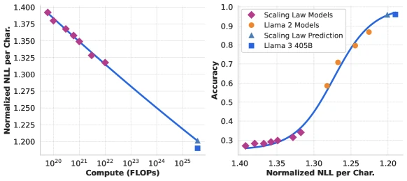
Figure 4 of The Llama 3 Herd of Models (arXiv:2407.21783), reproduced for editorial coverage.

---

MATH ENTRY 3: Direct Preference Optimization loss

• Source: Llama 3 paper Section 4.3 ² , applied per Rafailov 2023 ⁷ .
• What it is: The supervised loss that replaces the entire PPO-based RLHF stage during Llama 3 post-training.
• Formal definition:

$\mathcal{L}_{\text{DPO}}(\pi_\theta; \pi_{\text{ref}}) = -\mathbb{E}_{(x, y_w, y_l) \sim \mathcal{D}} \left[ \log \sigma \left( \beta \log \frac{\pi_\theta(y_w \mid x)}{\pi_{\text{ref}}(y_w \mid x)} - \beta \log \frac{\pi_\theta(y_l \mid x)}{\pi_{\text{ref}}(y_l \mid x)} \right) \right]$

• Each term:

  • $\pi_\theta$ is the trainable policy (the language model being post-trained); $\pi_\theta(y \mid x)$ is the probability the policy assigns to response $y$ given prompt $x$.
  • $\pi_{\text{ref}}$ is the frozen reference policy, typically the post-SFT model checkpoint.
  • $(x, y_w, y_l)$ is a preference triple: prompt $x$, preferred response $y_w$ (“winner”), dispreferred response $y_l$ (“loser”). $\mathcal{D}$ is the preference dataset.
  • $\beta$ is a temperature-like coefficient controlling how strongly the policy is anchored to the reference. Llama 3 uses $\beta = 0.1$ ² .
  • $\sigma$ is the sigmoid function $\sigma(z) = 1 / (1 + e^{-z})$.

• Worked numerical example. Suppose for a single preference pair, the log-probabilities are:

  • $\log \pi_\theta(y_w \mid x) = -10$, $\log \pi_{\text{ref}}(y_w \mid x) = -12$, so log-ratio $= 2$.
  • $\log \pi_\theta(y_l \mid x) = -15$, $\log \pi_{\text{ref}}(y_l \mid x) = -14$, so log-ratio $= -1$.

  Step 1: Compute the implicit-reward difference: $\beta \cdot (2 - (-1)) = 0.1 \cdot 3 = 0.3$.

  Step 2: Apply sigmoid: $\sigma(0.3) = 1 / (1 + e^{-0.3}) \approx 1 / (1 + 0.741) \approx 0.574$.

  Step 3: Loss for this pair: $-\log 0.574 \approx 0.555$.

  Step 4: Interpretation: the policy already prefers $y_w$ over $y_l$ relative to the reference (the gap is positive), so the loss is modest. Gradient descent will push the policy to widen the gap further.

• Role: The objective Llama 3 minimises during six iterative rounds of DPO post-training, each round using fresh human-annotated preference pairs.

• Edge cases: If $\beta \rightarrow 0$, the loss becomes insensitive to preferences (no learning signal); if $\beta \rightarrow \infty$, the policy moves arbitrarily far from the reference (regularisation lost). Llama 3’s choice of $\beta = 0.1$ is on the low end of the standard sweep range.

• Novelty: [Adopted] from DPO 2023 ⁷ ; [Adapted] by Llama 3 with two modifications: masking formatting tokens (special chat-template tokens not counted in the log-probability), and adding an NLL regularisation term with coefficient 0.2 on the chosen response.

• Why it matters: This single loss replaces what InstructGPT-era RLHF accomplished with a separately-trained reward model and PPO. The compute saving at frontier scale is large; the pipeline simplification is what enables six iterative rounds in the first place.

---

MATH ENTRY 4: Compute budget allocation in 4D parallelism

• Source: Llama 3 paper Section 3.3 ² .
• What it is: The decomposition of total training compute across four parallelism axes (tensor, context, pipeline, data).
• Formal definition: The total number of GPUs is the product

$N_{\text{GPU}} = \text{TP} \cdot \text{CP} \cdot \text{PP} \cdot \text{DP}$

where each factor is the degree of parallelism along that axis. For Llama 3 405B with 16,384 GPUs and CP=16, Meta’s configuration is roughly TP=8, CP=16, PP=16, DP=8 (the paper reports several settings; this is one cited point).

• Each term:

  • TP (tensor parallelism): splits matrix multiplications across GPUs.
  • CP (context parallelism): splits the sequence dimension across GPUs.
  • PP (pipeline parallelism): splits layers across GPUs.
  • DP (data parallelism, here FSDP / Fully Sharded Data Parallelism): replicates the model across GPU groups and shards optimizer state.

• Worked numerical example. Verify the product: $8 \cdot 16 \cdot 16 \cdot 8 = 16,384$. Correct.

  Per-GPU model state with TP=8, PP=16: each GPU holds $1 / (8 \cdot 16) = 1/128$ of the model parameters. For 405B, that’s $\sim 3.16$B parameters per GPU. At BF16 (2 bytes), parameter memory is $\sim 6.3$GB, leaving room for optimizer state, gradients, and activations within the 80GB HBM3 budget.

• Role: Determines whether a given model can be trained on the available cluster at all.

• Edge cases: The ordering [TP, CP, PP, DP] matters because network bandwidth is highest within a node (NVLink) and lowest across the cluster (InfiniBand); TP and CP are kept inside nodes where possible.

• Novelty: [Adapted] from Megatron-LM and FSDP; the specific combination at 16K-GPU scale with context parallelism is the contribution.

• Why it matters: Without this layout, the BF16 Model FLOPs Utilization of 38-43% reported in the paper would not be achievable, and the wall-clock training time would balloon.

---

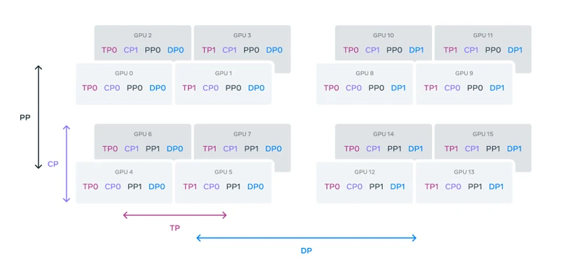
Figure 5 of The Llama 3 Herd of Models (arXiv:2407.21783), reproduced for editorial coverage.

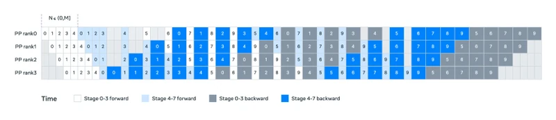
Figure 6 of The Llama 3 Herd of Models (arXiv:2407.21783), reproduced for editorial coverage.

7. Algorithmic contributions

ALGORITHM ENTRY 1: Llama 3 post-training round (iterative DPO)

• Source: Llama 3 paper Section 4 ² .
• Purpose: Produce the instruction-tuned model from the base model via six rounds of rejection-sampling-then-DPO.
• Inputs:
  • Base pretrained model $\pi_{\text{base}}$ (8B, 70B, or 405B)
  • Reward model $r_\phi$ trained on preference comparisons
  • Prompt corpus $\mathcal{P}$
  • Human-annotated preference dataset $\mathcal{D}_{\text{pref}}$ growing each round
• Outputs: Aligned instruction-tuned model $\pi_{\text{final}}$.

Pseudocode (faithful reconstruction; the paper does not publish line-by-line pseudocode):

def llama3_post_training(pi_base, r_phi, P, D_pref, rounds=6):
    pi = pi_base
    for t in range(rounds):
        # Step 1: SFT on filtered high-quality data
        sft_data = curate_sft_set(D_pref, target_size_t)
        pi = SFT(pi, sft_data, lr=1e-5, steps=8500)

        # Step 2: Rejection sampling
        rs_data = []
        for prompt in P:
            candidates = [sample(pi, prompt) for _ in range(K=10..30)]
            scores = [r_phi(prompt, c) for c in candidates]
            best = candidates[argmax(scores)]
            rs_data.append((prompt, best))

        # Step 3: DPO
        D_pref_t = collect_new_preferences(rs_data)
        D_pref = D_pref + D_pref_t
        pi = DPO(pi, pi_ref=pi, D=D_pref,
                 beta=0.1, lr=1e-5, nll_coef=0.2)

    return pi

• Hand-traced example on minimal input. Take rounds=2, $K=3$, prompts $\mathcal{P} = \{x_1, x_2\}$, and start with $\pi = \pi_{\text{base}}$.

  Round 1, Step 1: SFT on initial seed data; loss falls from, say, 2.3 to 1.4 over 8,500 steps. $\pi \rightarrow \pi^{(1)}_{\text{SFT}}$.

  Round 1, Step 2: For prompt $x_1$, sample 3 candidates $\{c_1, c_2, c_3\}$. Reward model scores $\{0.8, 0.3, 0.6\}$. Keep $c_1$. Same for $x_2$, keep best.

  Round 1, Step 3: Annotators rank $(c_1, c_2)$ and $(c_1, c_3)$ pairs. Preferences land in $\mathcal{D}_{\text{pref}}$. DPO loss runs over 100K-ish gradient steps; chosen-response log-prob rises by, say, +0.4 per token relative to reference; rejected-response log-prob falls by 0.3. $\pi \rightarrow \pi^{(1)}_{\text{DPO}}$.

  Round 2 repeats with updated $\pi$ and grown $\mathcal{D}_{\text{pref}}$. The reward model is also iteratively improved; Meta does not publish exactly how synchronised the reward-model updates are with the policy rounds.

• Complexity: Each round costs roughly one SFT pass (proportional to SFT-set size) plus rejection-sampling generation cost ($\mid \mathcal{P}\mid \cdot K$ generations) plus DPO gradient steps. Six rounds at 405B scale is a multi-week post-training run.

• Hyperparameters: SFT learning rate $10^{-5}$, SFT steps 8,500-9,000, DPO learning rate $10^{-5}$, DPO $\beta = 0.1$, NLL regularisation 0.2, $K \in [10, 30]$ rejection-sampling candidates.

• Failure modes: Reward hacking (the policy finds responses that fool the reward model without being genuinely better); preference dataset drift (early-round preferences may not transfer to later-round policy distributions).

• Novelty: [Adapted]. SFT, rejection sampling, and DPO each predate Llama 3; the iterative six-round cocktail at frontier scale is the specific contribution.

ALGORITHM ENTRY 2: Llama 4 MoE forward pass

• Source: Llama 4 blog ³ and Hugging Face model cards ^{4 5} . [Reconstructed] Exact routing implementation not published; this is the standard MoE forward pass adapted to the alternating-dense pattern.
• Purpose: Process one token through one MoE layer.
• Inputs: Token representation $x \in \mathbb{R}^`{d}`$, expert weights $\{W_e\}_{e=1}^`{E}`$, gating projection $W_g \in \mathbb{R}^{E \times d}$, top-$k$.
• Outputs: Updated token representation $y \in \mathbb{R}^`{d}`$.

Pseudocode (reconstructed):

def moe_layer_forward(x, experts, W_g, k):
    gates = softmax(W_g @ x)         # length-E vector
    topk_indices = topk(gates, k)     # k expert IDs
    topk_gates = gates[topk_indices]  # k weights
    topk_gates = topk_gates / topk_gates.sum()  # renormalize
    y = 0
    for i, e in enumerate(topk_indices):
        y = y + topk_gates[i] * experts[e](x)
    return y

• Hand-traced example. See MATH ENTRY 2’s worked example for the gating numerics; the algorithmic structure adds the renormalisation step (top-$k$ gates summed to 1) and the actual expert evaluations.

• Complexity: Per token, $k$ expert FFN evaluations plus the gating projection. For Scout ($E=16$, $k$ likely 2), the compute is $\sim 2/16 = 12.5\%$ of a dense model with the same total expert capacity. Memory for all $E$ experts is held in GPU memory; only $k$ are computed.

• Hyperparameters: $E = 16$ (Scout) or 128 (Maverick); $k$ not officially disclosed but standard MoE practice and the “alternating dense and MoE layers” framing ³ suggest $k = 1$ or $k = 2$. [Reconstructed]

• Failure modes: Load imbalance across experts if the auxiliary balancing loss is mis-tuned; expert collapse if routing concentrates on a few experts during early training.

• Novelty: [Adopted].

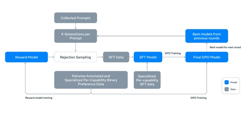
Figure 7 of The Llama 3 Herd of Models (arXiv:2407.21783), reproduced for editorial coverage.

8. Specialised design contributions

Subsection 8A, LLM / prompt design. Not applicable to this paper. Llama 3 and Llama 4 are base models plus post-training; the post-training procedure is described in MATH ENTRY 3 and ALGORITHM ENTRY 1 rather than as a prompt-engineering contribution.

Subsection 8B, architecture-specific details.

• Llama 3: GQA with 8 KV groups across all sizes (8B, 70B, 405B); SwiGLU FFN; RMSNorm pre-norm; RoPE base 500K; tied input/output embeddings on the 8B variant, untied on 70B and 405B. Context-length staging: 8K base, then six incremental stages to 128K, then final annealing ² .
• Llama 4: Alternating dense and MoE feed-forward layers (the attention layers remain dense). Early fusion for vision (image patches projected directly into token stream). iRoPE for Scout’s 10M-token context: some layers use RoPE, others use no positional encoding; inference-time temperature scaling on attention logits compensates for the long-context attention dilution ³ .

Subsection 8C, training specifics.

• Llama 3: 16,000 H100 GPUs at 700W TDP with 80GB HBM3 ² . BF16 precision. 4D parallelism (TP / CP / PP / FSDP) with ordering [TP, CP, PP, DP] optimised for the InfiniBand topology. Achieved MFU 38-43% depending on parallelism degree. Data mixture: 50% general knowledge, 25% math/reasoning, 17% code, 8% multilingual. Data annealing at the very end: final 40M tokens with learning rate linearly decayed to zero and high-quality sources upsampled; final checkpoint is the average across the annealing window ² .
• Llama 4: “More than 30 trillion tokens, more than double the Llama 3 pre-training mixture” ³ . FP8 precision training reportedly achieving 390 TFLOPs/GPU at 32,000-GPU scale ³ . Pre-trained on 200 languages, over 100 with $\geq 1$ billion tokens each. [Reconstructed] Exact GPU count for Llama 4 (vs. the 32K figure for the FP8 throughput claim, which may be a subset) is not disclosed.

Subsection 8D, inference / deployment specifics.

• Llama 3 405B: Designed to be servable in BF16 on $8 \times$ H100 80GB or in FP8 on 4 GPUs; the KV cache at 128K context is the binding constraint for serving long-context requests.
• Llama 4 Maverick: “Can be run on a single NVIDIA H100 DGX host” ³ (8 GPUs, 640GB HBM total). The MoE design’s whole point: 400B total parameters but per-token compute equivalent to a 17B dense model.
• Llama 4 Scout: Marketed as running on a single H100 GPU at appropriate quantisation. The 10M-token context window is a stress capability, not a quality guarantee at full context; [Reviewer Perspective] independent evaluations at launch reported quality degradation well below 10M tokens.

9. Experiments and results

Datasets and benchmarks (Llama 3). Meta evaluates on the standard public suite: MMLU (massive multitask language understanding), HumanEval (Python code), MBPP (Python code), GSM8K (grade-school math), MATH (competition math), ARC-Challenge (reasoning), TriviaQA (factual QA), MultiPL-E (multilingual code), and several long-context benchmarks (Needle-in-a-Haystack, ZeroSCROLLS).

Baselines. GPT-4 0125, Claude 3.5 Sonnet, Gemini 1.5 Pro, Mixtral 8x22B for the open-weights comparison, plus Llama 2 70B as the predecessor.

Reproduced key results (Llama 3 405B Instruct).

Benchmark	Llama 3 405B	GPT-4 (0125)	Claude 3.5 Sonnet
MMLU (5-shot)	87.3	85.1	89.9
HumanEval	89.0	86.6	92.0
GSM8K (8-shot)	96.8	94.2	96.4
MATH (0-shot)	73.8	64.5	71.1
ARC Challenge	96.9	96.4	96.7

Table 2 of The Llama 3 Herd of Models (arXiv:2407.21783), reproduced for editorial coverage. ¹

Main quantitative results. Llama 3 405B sits competitive-to-slightly-behind Claude 3.5 Sonnet on MMLU and HumanEval, ahead of GPT-4 0125 on MMLU + GSM8K + MATH, roughly tied across reasoning benchmarks. [Analysis] The MATH score (73.8 vs. GPT-4’s 64.5) is the most striking gap and reflects Meta’s data-mixture emphasis on math and reasoning tokens (25% of the corpus).

Llama 4 benchmark results. [From the paper, hedged] ³ Meta claims Maverick beats GPT-4o and Gemini 2.0 Flash on the evaluation suite reported in the launch blog. Behemoth is claimed to beat GPT-4.5, Claude Sonnet 3.7, and Gemini 2.0 Pro on STEM benchmarks while still in training. [Reviewer Perspective] Independent reproducibility was contested at launch; Nathan Lambert’s Interconnects analysis flags evaluation-harness choices and the gap between the variants Meta benchmarked and the variants released to Hugging Face ¹² .

Ablations (Llama 3). The paper reports ablations on data mixture (showing the math-reasoning slice is the most quality-sensitive), on the number of DPO rounds (with diminishing returns after round 4), on rejection-sampling $K$ (saturating around $K=20$), and on context-extension stage count. Hyperparameter sensitivity is documented for SFT learning rate, DPO $\beta$, and the NLL regularisation coefficient.

Robustness / stress tests. Llama 3 reports Needle-in-a-Haystack performance staying high through 128K context. Llama 4 Scout reports the same at 10M context; [Reviewer Perspective] independent NiaH results vary widely depending on needle placement and noise content.

Qualitative results. The Llama 3 paper includes appendix examples of long-context QA, code translation, and multilingual generation. Llama 4 emphasises multimodal use cases (image-grounded chat) at launch.

Experimental scope limits. Llama 3’s evaluation is text-only for the released 405B; the multimodal (vision, video, speech) capabilities are described as “not yet broadly released” in the paper itself, with the Llama 3.2 vision adapter shipping later separately. Llama 4’s evaluation harness at launch was contested ([Reviewer Perspective] see Section 11).

Independent benchmark cross-check. For Llama 3, the LMSYS Chatbot Arena results (publicly visible at lmarena.ai) provide a community-driven cross-check that broadly agrees with the paper’s positioning. For Llama 4 Maverick, the initial Chatbot Arena leaderboard placement was high but was subsequently disputed when Meta’s submitted variant turned out to differ from the publicly released checkpoint; the Interconnects analysis ¹² documents this. Treat the SOTA claim as the authors’ framing on their chosen benchmark suite; independent reproducibility has been partial.

Evidence audit [Analysis].

• Strongly supported: Llama 3 scaling-law derivation; data mixture; MFU statistics; hardware-failure statistics; quantitative benchmarks reproducible from Hugging Face weights.
• Partially supported: Llama 4 Maverick benchmarks (depends on which checkpoint is used); Llama 4 Scout 10M context (passes synthetic tests, less clear on real workloads).
• Narrow evidence: Llama 4 Behemoth claims (still training at announcement; no released weights).

10. Technical novelty summary

Component	Type	Novelty	Justification	Source
Llama 3 scaling-law fit	Combination	Incrementally novel	Refits Chinchilla at Meta’s data mixture; $\alpha = 0.53$ specific to the run	2
Llama 3 6-round iterative DPO	Combination	Combination novel	Combines rejection sampling + DPO + NLL reg iteratively at frontier scale	2
Llama 3 4D parallelism at 16K GPUs	Combination	Combination novel	TP + CP + PP + FSDP at unprecedented scale; CP adds new axis for long context	2
Llama 4 iRoPE for 10M context	Fully novel	Fully novel ([Reconstructed])	Interleaved RoPE / no-positional layers with inference-time temperature scaling	3
Llama 4 MoE design	Adopted	Adopted	Standard MoE post-Switch and Mixtral; Meta’s contribution is scale + alternating dense layout	3
Llama 4 early-fusion multimodality	Adapted	Incrementally novel	Vision-token-into-stream pattern adopted from Fuyu / Chameleon; Meta’s commitment is the integration into the full training corpus	3
Llama 4 distillation from Behemoth	Adapted	Incrementally novel	Distillation is standard; “dynamic soft/hard target weighting” framing is Meta-specific	3

Single most novel contribution. [Analysis] The Llama 3 paper’s contribution is not a new architectural idea; it is the rigour and transparency of the scaling-law-driven design choice at frontier scale, paired with the most detailed public account of post-training to date. The Llama 4 release’s contribution is the architectural pivot itself: Meta’s commitment that future frontier open-weights models are sparse, not dense.

What the papers do NOT claim novel. GQA, RoPE, RMSNorm, SwiGLU, DPO, rejection sampling, SFT, MoE routing, top-$k$ gating, early-fusion multimodality, and the H100-cluster infrastructure are all adopted from prior work.

11. Situating the work

What prior work did. Chinchilla ⁶ established that model size and training tokens should grow together with compute; prior frontier models (GPT-3, PaLM, Llama 2) were widely held to be undertrained on tokens. Switch Transformer ⁹ and Mixtral ¹⁴ established that MoE at scale is viable for language modelling. DPO ⁷ simplified RLHF away from PPO. Compositional multimodal designs (LLaVA-style) preceded native early-fusion designs (Fuyu, Chameleon).

What Llama 3 + Llama 4 change conceptually. [Analysis] Llama 3 normalises Chinchilla-scaling-by-rigour as the open-weights expectation: any future frontier release that does not document its scaling-law derivation will be conspicuously absent that piece. Llama 4 normalises MoE-with-active-parameter-budget-disclosure: future open-weights releases will be compared on $N_a$ (active) not just $N_t$ (total). The compute-vs-quality and cost-vs-quality Pareto frontiers shift in the open-weights ecosystem.

Contemporaneous related work.

• DeepSeek-V3 (December 2024) ¹³ : 671B total / 37B active MoE; reported training cost ~$5.6M; competitive on benchmarks with Llama 3 405B at a fraction of the compute. [External comparison] Almost certainly the unstated competitive context for Meta’s MoE pivot to Llama 4.
• Mixtral 8x22B (April 2024) ¹⁴ : 141B total / 39B active MoE; predecessor MoE that established the open-weights MoE pattern.

[Reviewer Perspective] Strongest skeptical objection. The Llama 4 release’s transparency dropped sharply relative to Llama 3. Where Llama 3 published a 90+-page technical report with scaling-law derivations and full hyperparameter tables, Llama 4 shipped with a blog post, model cards, and contested benchmark-harness choices ¹² . The “Llama 4” badge inherits trust the Llama 3 paper built; the Llama 4 release does not earn that trust on its own published disclosure.

[Reviewer Perspective] Strongest author-side rebuttal. The Llama 4 release is a product launch, not an academic paper; the model cards plus weights plus Hugging Face availability are the artefacts that matter for downstream users. The technical report can follow.

What remains unsolved.

• Whether the Llama 3 scaling law extrapolates beyond $10^{26}$ FLOPs.
• Whether 10M-token context in MoE models is useful in practice or only on synthetic stress tests.
• Whether early-fusion multimodality scales as cleanly as dense-text scaling laws.
• Whether the six-round DPO recipe transfers to MoE post-training without modification (Llama 4 reportedly uses “online RL” between SFT and DPO ³ , suggesting it did not).

Three future research directions.

1. Publication of the actual Llama 4 technical report with the scaling-law derivation, data-mixture disclosure, and post-training hyperparameters at the rigour of the Llama 3 paper. [Analysis] The most-requested artefact among practitioners building on Llama 4.
2. Decoupling of “training compute” from “active-parameter compute” in scaling laws for MoE; the dense $C \approx 6 N D$ accounting does not transfer cleanly.
3. Independent reproducibility studies for Llama 4 Maverick’s reported benchmark wins on a transparent harness with the publicly-released weights.

12. Critical analysis

Strengths (Llama 3).

• Unmatched disclosure depth for a frontier-scale training run; scaling-law derivation, data mixture, post-training recipe, hardware-failure statistics all in one document.
• Reproducibility: weights are openly available on Hugging Face; the post-training recipe is documented well enough to be implemented from the paper.
• Quality: 405B competitive with closed frontier models on math, reasoning, and code benchmarks.

Weaknesses explicitly stated by the authors (Llama 3). Multimodal capabilities (“image, video, speech”) were “not yet broadly released” at paper publication time ¹ ; safety classifier Llama Guard 3 details are deferred to a separate technical artefact; training data sources are not enumerated (the mixture percentages are disclosed but not the underlying corpora).

Weaknesses not stated by the authors [Reviewer Perspective].

• Data provenance: the corpus is not publicly auditable; reproduction without Meta’s data is not possible.
• Reward-model architecture: the reward model trained for rejection sampling and DPO preference annotation is not architecturally described.
• Llama 4 specifically: the disclosure level dropped, the benchmark-harness was contested, and the launched Hugging Face variants differed from the variants Meta benchmarked ¹² .

Reproducibility check.

Artefact	Status (Llama 3)	Status (Llama 4)
Code (training)	Not released; recipe documented in paper	Not released
Code (inference)	Released via Hugging Face transformers	Released via Hugging Face transformers
Data (pretraining)	Not released	Not released
Hyperparameters	Fully disclosed in paper	Partially disclosed in blog and model cards
Compute	Reported (16K H100s)	Partially reported (32K-GPU FP8 throughput; total not explicit)
Trained weights	Released (huggingface.co/meta-llama)	Released (Scout + Maverick); Behemoth not released
Evaluation set	Public benchmarks; standard harnesses	Public benchmarks; harness choice contested
Overall	Partially reproducible	Less reproducible

Methodology disclosure.

• Sample size: 15.6T pretraining tokens (Llama 3 405B); $>30$T (Llama 4). Post-training preference dataset size: not publicly enumerated, but the Table 6 distribution in the Llama 3 paper documents proportions.
• Evaluation set: Standard public benchmarks (MMLU, HumanEval, GSM8K, MATH, ARC). Contamination check: Meta runs a 13-gram contamination filter and reports the impact; the paper documents this.
• Baselines: GPT-4 0125, Claude 3.5 Sonnet, Gemini 1.5 Pro, Mixtral 8x22B (Llama 3); GPT-4o, Gemini 2.0 Flash (Llama 4 launch).
• Hardware / compute: 16,000 H100 GPUs for Llama 3; 32K-GPU FP8 throughput cited for Llama 4 without a single end-to-end compute figure.

Generalisability. The Llama 3 post-training recipe transfers to any decoder-only Transformer with preference data; teams have already adopted iterative DPO with NLL regularisation on smaller bases. The Llama 4 MoE design transfers more conditionally; the alternating-dense pattern, the iRoPE long-context recipe, and the early-fusion multimodal integration each carry distinct engineering costs.

Assumption audit. The Chinchilla scaling assumption is load-bearing; if the extrapolation from $10^{22}$ to $3.8 \times 10^{25}$ FLOPs were misfit, the optimal model could be substantially under- or over-sized. The benchmark-quality-correlates-with-loss assumption is load-bearing for the entire methodology of using small-scale loss measurements to pick large-scale architectures. Both assumptions held in the Llama 3 result; whether they continue to hold at the next order of magnitude is open.

What would make the papers significantly stronger. [Analysis]

• A formal Llama 4 technical report at Llama 3’s rigour.
• Open release of the pretraining data, or at minimum a structured data card listing sources and licences.
• Public release of the reward-model architecture and training data.
• An independent reproducibility harness for the Llama 4 benchmark claims.

13. What is reusable for a new study

REUSABLE COMPONENT 1: The Chinchilla-style scaling-law fitting procedure. Run isoFLOP experiments across a 4-order-of-magnitude compute range at small scale; fit a power law for compute-optimal model size; extrapolate to the target budget. Llama 3 shows this works at frontier scale. Preconditions: a clean small-scale training pipeline and a clean loss measurement at multiple $(N, D)$ pairs. Risks: the extrapolation gap. Suitable for any team training a foundation model at sufficient scale.

REUSABLE COMPONENT 2: The 6-round iterative DPO recipe. SFT then rejection sampling then DPO, repeated. Llama 3’s hyperparameters (SFT LR $10^{-5}$, DPO $\beta = 0.1$, NLL coefficient 0.2, $K = 10$-$30$) are documented at frontier scale and transfer to smaller bases. Preconditions: a reward model and a growing preference dataset. Risks: reward hacking; preference dataset drift across rounds.

REUSABLE COMPONENT 3: Long-context staging. RoPE base 500K, then six incremental context-extension stages, then annealing. Llama 3’s recipe is the most rigorous published long-context extension procedure. Preconditions: a strong short-context base. Risks: training-data quality at long contexts matters more than at short.

REUSABLE COMPONENT 4: The data-annealing trick at end of training. Final 40M tokens with learning rate linearly decayed to zero, high-quality sources upsampled, final checkpoint averaged across the annealing window. Cheap, transferable, no architectural changes required.

REUSABLE COMPONENT 5: Llama 4’s alternating-dense-and-MoE layer layout. Reduces the implementation complexity of pure MoE (where every FFN is MoE); some layers stay simple. Preconditions: an MoE training infrastructure. Risks: the alternation ratio is a hyperparameter Meta does not publicly disclose.

Dependency map. Component 1 (scaling laws) is upstream of every other choice. Component 3 (long-context staging) depends on Component 1 having sized the base correctly. Component 2 (iterative DPO) depends on a reward model trained on preferences; Component 4 (data annealing) is independent of post-training. Component 5 (alternating MoE) is independent of all of Components 1-4 and can be added to any dense-Transformer recipe.

Recommendation. [Analysis] The three highest-value components for teams building new foundation models in 2026: the scaling-law procedure (Component 1), the iterative DPO recipe (Component 2), and the data-annealing trick (Component 4). The MoE layout (Component 5) is reusable but requires more infrastructure than most teams have.

What type of new study benefits most. A team training an open-weights base model at $\geq 10$B parameters and $\geq 1$T tokens, with a clear deployment target, can use this multi-paper combination as the recipe scaffold.

14. Known limitations and open problems

Limitations explicitly stated by the authors (Llama 3). Multimodal capabilities deferred. Safety-classifier details deferred. Data sources not enumerated. Reward-model architecture not detailed. Long-context evaluation focuses on synthetic Needle-in-a-Haystack rather than full-context downstream task quality.

Limitations not stated (Llama 4) [Analysis] + [Reviewer Perspective]. Benchmark-harness choices contested at launch ¹² . Launched Hugging Face variants differed from Meta’s benchmark variants. iRoPE 10M-context claim relies on inference-time tricks (attention temperature scaling) whose generalisation is not independently verified. No formal technical report at release.

Technical root cause of each.

• Disclosure gap: a product-launch decision, not a technical constraint.
• Benchmark-harness gap: incentive misalignment between launch optics and reproducible evaluation.
• iRoPE generalisation: an open empirical question about how well synthetic long-context tasks correlate with real long-context quality.

Open problems.

• A unified scaling law for MoE that accounts for both active-parameter compute and total-parameter memory.
• Whether the iterative DPO recipe transfers to MoE post-training as-is, or requires the “online RL” stage Meta added in Llama 4 ³ .
• Whether early-fusion multimodality scales as cleanly as text scaling laws suggest.

What a follow-up paper would need. [Analysis] The single most useful follow-up would be a formal Llama 4 technical report at Llama 3’s rigour, with the scaling-law fits for MoE specifically, the post-training recipe end-to-end, and a contamination-checked benchmark harness whose results are reproducible from the released weights.

How this article reads at three depths

For the curious high-school reader. Llama 3 and Llama 4 are Meta’s two latest “open weights” big language models. Llama 3 is a giant single network with 405 billion adjustable numbers, trained on roughly 15 trillion words of text. Llama 4 splits its 400 billion numbers into a panel of experts and uses only a few experts per word, which is cheaper to run while still being powerful. The papers behind these models are the most detailed public account of how to build something at this scale.

For the working developer or ML engineer. Llama 3’s value is the fully-documented Chinchilla-scaling-law-driven design plus the iterative SFT-rejection-sampling-DPO post-training recipe; both transfer to smaller bases and are the most rigorous public reference for either. Llama 4’s value is the MoE deployment profile: 400B total parameters running on a single H100 DGX node at the per-token compute of a 17B dense model, plus early-fusion multimodal integration. Trade-offs: Llama 4’s disclosure level is much lower than Llama 3’s, the launched checkpoints differed from the benchmarked ones at release, and the 10M-token context window relies on inference-time tricks of unclear robustness. For a new build today, Llama 4 is the default for multimodal; Llama 3 405B is the default when reproducibility against the paper matters.

For the ML researcher. The Llama 3 paper’s central contribution is rigour: the scaling-law derivation $N^{*}(C) = 0.29 \cdot C^{0.53}$ fit on isoFLOPs from $6 \times 10^{18}$ to $10^{22}$ FLOPs and extrapolated to $3.8 \times 10^{25}$ FLOPs, plus the six-round iterative DPO recipe with $\beta = 0.1$ and NLL regularisation 0.2. Llama 4’s contribution is the architectural pivot: alternating dense and MoE layers, iRoPE for 10M context, early-fusion multimodality, FP8 training at 32K-GPU scale. The load-bearing assumption across both is that small-scale loss measurements predict large-scale benchmark quality; both releases support that assumption empirically but not theoretically. The strongest objection is the asymmetry in disclosure: Llama 3 set a publication bar that Llama 4 has not yet met. A follow-up paper publishing the formal Llama 4 technical report at Llama 3’s rigour would close the highest-payoff gap in the open-weights frontier-model literature today.