IBM's Granite open-model lineage — a multi-paper review

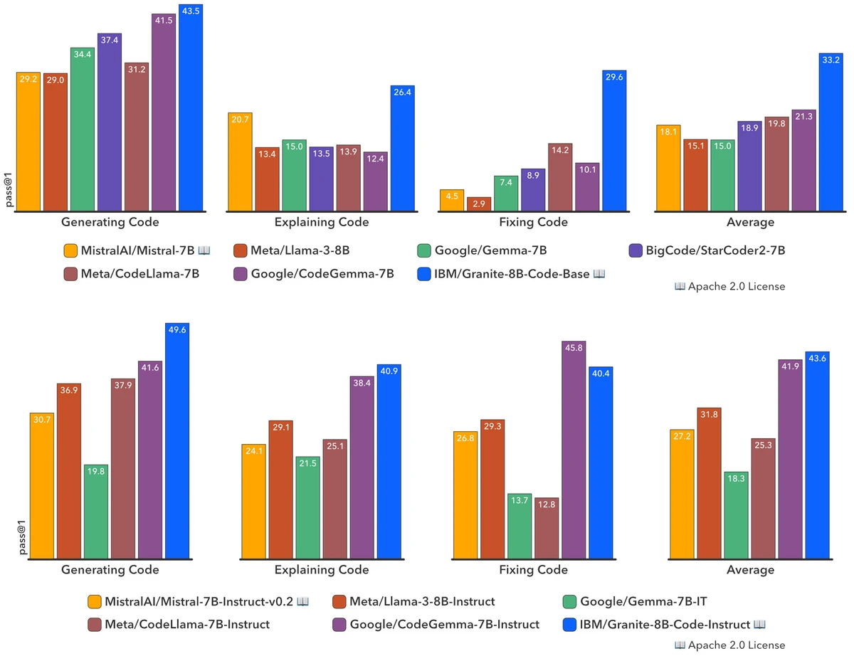
Figure 1 of Granite Code Models (arXiv:2405.04324), reproduced for editorial coverage.

1. Umbrella scope and paper identity

Citations.

• Mishra et al., “Granite Code Models: A Family of Open Foundation Models for Code Intelligence,” arXiv:2405.04324, May 2024 ¹ . The flagship code-specialised release with base + instruct variants at 3B, 8B, 20B and 34B parameters.
• Ekambaram et al., “Tiny Time Mixers (TTMs): Fast Pre-trained Models for Enhanced Zero/Few-Shot Forecasting of Multivariate Time Series,” arXiv:2401.03955, accepted at NeurIPS 2024 ^{3 4} . The compact pretrained time-series stack later released under the Granite-TimeSeries brand.
• Granite Team, IBM, “Granite 3.0 Language Models,” technical report bundled with the October 2024 release on GitHub ⁵ . The third-generation general-purpose language-model release covering Dense 2B + 8B and Mixture-of-Experts 1B-A400M + 3B-A800M variants.

Retrieval. The Granite Code Models paper was retrieved in full via the ar5iv HTML render ² . The TTM paper was retrieved via the arXiv abstract plus the NeurIPS 2024 proceedings landing page ^{3 4} ; full benchmark tables were reconciled against the official Hugging Face model card for the R2 release ⁸ . The Granite 3.0 technical report PDF on the official ibm-granite/granite-3.0-language-models GitHub repository ⁵ was not text-extractable via automated fetch on the writing date; this article reconstructs the Granite 3.0 architecture and training-recipe details from the official Hugging Face model cards ^{6 7} , the IBM newsroom launch post ⁹ , and the closely-associated Power Scheduler paper ¹⁰ from the same Granite team, with reconstructed material flagged inline. The Granite Guardian safety model card ¹¹ grounds the safety-stack discussion in Section 12.

Classification. Architecture proposal (the TTM multilevel patch-mixer backbone; Granite 3.0 MoE routing), training method (two-phase pretraining recipe shared across all three releases; FIM objective for Code Models; Power Scheduler for Granite 3.0), benchmark (HumanEvalPack, MBPP+, MultiPL-E for code; standard time-series benchmarks for TTM; HELM-style aggregate benchmarks for Granite 3.0). Granite 3.0 and the Code Models are LLM-based; TTM is a purpose-built non-LLM forecasting foundation model and reads more like a representation-learning paper than a generative-model paper.

Technical abstract in the publication’s voice. This article reviews three releases that together form IBM’s enterprise-oriented open-weights stack as of late 2024 into 2026. The Granite Code Models paper documents a four-size code-specialised family (3B / 8B / 20B / 34B), trained in two phases on 4.5 trillion tokens drawn from 116 programming languages plus mixed natural-language data, released under Apache 2.0 with both base and instruction-tuned variants and with the 34B model produced via depth upscaling from the 20B checkpoint after 1.6T tokens. The TTM paper proposes a sub-million-parameter pretrained multivariate time-series forecaster built on the TSMixer MLP-mixer backbone with adaptive patching, diverse resolution sampling and resolution prefix tuning, and shows zero-shot and few-shot wins on standard horizons (96, 192, 336, 720) against larger transformer baselines. The Granite 3.0 technical report covers IBM’s third-generation general-purpose language models: a Dense 2B and Dense 8B paired with two MoE variants (1B-total / 400M-active and 3B-total / 800M-active), all trained on a two-stage 10T-to-12T-token recipe across twelve natural languages and 116 programming languages on IBM’s Blue Vela H100 cluster ^{6 7 9} .

Primary research questions.

• Granite Code: Can a smaller open-weights code-specialised family trained on rigorously filtered code data match or exceed the much larger CodeLlama and StarCoder2 families on standard code benchmarks while shipping under Apache 2.0?
• TTM: Can a sub-million-parameter pretrained model beat billion-parameter time-series foundation models on zero-shot multivariate forecasting?
• Granite 3.0: Can IBM’s enterprise-tuned training recipe (the Power Scheduler, two-stage data mix, MoE routing, safety alignment via Granite Guardian) produce same-class quality at notably smaller active-parameter counts than the Llama and Qwen open-weights baselines?

Core technical claims.

• Granite Code: Granite-8B-Code-Base beats CodeLlama-7B on 16 of 18 MultiPL-E languages and beats CodeGemma-8B by 12 points on HumanEvalPack (33.2% vs 21.3%); the 8B model beats CodeLlama-34B by 9.3% on HumanEvalExplain ² .
• TTM: The 1M-parameter TTM-R2 family outperforms TimesFM, Chronos, Moirai, Lag-Llama, Moment, GPT4TS, TimeLLM and LLMTime on standard zero-shot forecasting benchmarks and runs on CPU ⁸ .
• Granite 3.0: Two-stage training across 10T (stage 1) and 2T (stage 2) tokens with the Power Scheduler and the Blue Vela H100 cluster produces a Dense 8B that scores 65.54% on MMLU and 52.44% on HumanEval at the base checkpoint ⁶ , while the MoE 3B-A800M activates only 800M parameters per token at inference ⁷ .

Core technical domains.

Domain	Depth
Open-weights language-model pretraining	deep
MoE routing and sparse-expert training	moderate
Code-specialised pretraining and FIM	deep
Multivariate time-series foundation models	deep
MLP-mixer architectures	moderate
Power-law learning-rate scheduling	moderate
Safety alignment via separate guardian model	surface

Reader prerequisites. High-school algebra is enough to follow the on-ramp. Familiarity with neural-network basics (attention, embedding, softmax) is helpful but not required because the Glossary in Section 2.5 covers them. The TTM section assumes the reader knows what a time series is; the Glossary covers MLP-mixer, patching and channel-mixing. The Granite 3.0 MoE discussion assumes the reader has read about Mixture-of-Experts; Glossary covers top-k routing.

2. TL;DR and executive overview

TL;DR. IBM has spent 2024 and early 2026 shipping a stack of open-weights models under the Granite brand: language models, code models, and a tiny time-series forecaster, all released under the same Apache 2.0 license that lets anyone use them commercially. The lineage is built around a clear enterprise pitch: smaller than the Llama and Qwen models you read about most, but trained on more carefully filtered data, and bundled with a separate safety model called Granite Guardian so that production deployments can ship with guardrails. This article walks through the three landmark papers behind the lineage, explains the math and the algorithms in plain language with worked examples, and flags where IBM’s claims hold up against independent evidence and where the reader should hedge.

Executive summary. Three releases anchor the Granite stack as of 2026. The Code Models paper (May 2024) ships a four-size code-specialised family at 3B / 8B / 20B / 34B parameters, trained on 4.5 trillion code-and-language tokens across 116 programming languages, with both completion and fill-in-the-middle objectives. The TTM paper (NeurIPS 2024) ships a sub-million-parameter time-series forecaster built on the TSMixer MLP-mixer backbone that beats much larger transformer baselines in zero-shot settings and runs on a laptop CPU. The Granite 3.0 release (October 2024) ships a four-variant general-purpose language family (two dense at 2B and 8B, two MoE at 1B-A400M and 3B-A800M), trained on a two-stage 10T-to-12T-token recipe with the team’s own Power Scheduler. All three carry Apache 2.0; all three target enterprise use cases (RAG, function calling, cybersecurity, code, forecasting) rather than chat leaderboards. Working developers should read this article if they are picking a smaller open-weights model to self-host; ML researchers should read it for the depth-upscaling, MoE-routing and adaptive-patching details.

Five practitioner-relevant takeaways.

• The Granite Code 8B variant is the strongest 7-to-8B-class open-weights code model on HumanEvalPack as of mid-2024; for ≤16GB GPU self-hosting it is a serious alternative to CodeLlama-7B and StarCoder2-7B.
• The Granite 3.0 8B Dense scores 65.54% on MMLU at the base checkpoint per its HuggingFace card, putting it in roughly the same neighbourhood as Llama-3.1-8B-Base for general knowledge without matching the Llama post-training polish.
• TTM is the only sub-million-parameter pretrained forecaster in the open-weights landscape; if your forecasting workload is on-prem and CPU-only, TTM matters more than the size suggests.
• Granite Guardian is sold as the safety layer for production deployments, because Granite 3.0 base models explicitly carry no safety alignment per their model cards.
• The two MoE variants (1B-A400M and 3B-A800M) ship as 32-and-40 expert designs with 8-way top-k routing; active-parameter cost at inference is the headline metric IBM optimises.

Pipeline overview (training-time vs inference-time). All three releases share a common training-time pattern: pretraining on a curated mixed-domain corpus, optional second stage on higher-quality data, optional instruction tuning, optional DPO or model souping. TTM departs from this in detail (it is pretrained on raw time-series data with channel-independence and adaptive patching, then optionally fine-tuned with exogenous covariates), but the meta-pattern is the same: a substrate of pretraining followed by lightweight specialisation. Inference-time, the Code Models and Granite 3.0 dense variants are standard decoder-only transformer rollouts; the MoE variants add a top-k expert-routing pass per token; TTM runs a single forward pass through the mixer backbone followed by the decoder head.

2.5 Glossary

Term	Plain-English explanation	First appears in
Token	A small chunk of text (roughly a word fragment) the model reads or writes. A 12-trillion-token training run means the model saw 12 trillion such chunks.	Section 1
Pretraining	The big initial training phase that teaches the model the structure of language and code from huge amounts of raw text.	Section 1
Instruction tuning	A shorter follow-up training phase that teaches the pretrained model to follow human instructions.	Section 1
Mixture of Experts (MoE)	A model architecture that contains many small expert sub-networks and routes each input token to only a few of them, so the model is large in total but cheap per token.	Section 1
Top-k routing	The MoE rule that picks the top k experts (e.g., top 8 out of 40) for each token and ignores the rest.	Section 5C
Active parameters	The subset of an MoE model’s weights actually used for a given token, as opposed to total parameters which counts all experts.	Section 5C
Grouped Query Attention (GQA)	An attention variant that gives multiple query heads the same key-value head, cutting memory cost at small quality loss.	Section 5A
Rotary Position Embedding (RoPE)	A way of telling the transformer where each token sits in the sequence by rotating the query and key vectors.	Section 5A
Fill-in-the-Middle (FIM)	A training objective where the model sees prefix + suffix and must produce the middle, useful for code completion.	Section 6
TSMixer	An MLP-mixer architecture for time series — instead of attention, it uses small feed-forward networks that alternately mix across time-patches and channels.	Section 7B
Adaptive patching	TTM’s trick of changing patch length and patch count from layer to layer to capture both fine-grained and coarse-grained time structure.	Section 7B
Channel mixing	The operation that lets a multivariate time-series model share information across different signal channels.	Section 7B
Zero-shot forecasting	Forecasting on a dataset the model has never seen during pretraining, with no fine-tuning.	Section 9
Depth upscaling	Building a deeper model by duplicating layers from a shallower trained checkpoint, then continuing training.	Section 5A
Power Scheduler	A learning-rate schedule from the same IBM Granite team that picks the optimal learning rate based on a power-law in batch size and training-token count.	Section 6
HumanEvalPack	A code benchmark that extends OpenAI HumanEval to six languages and three task types (synthesise, explain, fix).	Section 9
MultiPL-E	A code benchmark that translates HumanEval-style problems into 18 programming languages.	Section 9
Granite Guardian	A separate IBM-trained model used as a safety classifier on top of Granite 3.0 base models.	Section 12
[Analysis] label	The publication’s own reasoned assessment, distinct from what the paper claims.	Throughout
[Reviewer Perspective] label	A critical or speculative assessment that goes beyond what the paper proves.	Sections 11–12
[Reconstructed] label	Content the publication faithfully reconstructed because the original artefact was only partially accessible.	Throughout
[External comparison] label	A comparison to prior or contemporaneous work outside the three papers under review.	Sections 4 + 11
”From the paper:” prefix	Content directly supported by the paper’s text, tables, or figures.	Throughout

3. Problem formalisation

Three distinct problems sit under the umbrella, but they share IBM’s enterprise framing: open-weights, Apache-licensed, smaller than the Meta and Alibaba flagships, with the data provenance documented.

3A. Granite Code Models. From the paper: the problem is supervised pretraining of a decoder-only transformer $f_\theta : \mathcal{V}^{*} \to \mathcal{V}^{*}$ on a code-heavy mixture, where $\mathcal{V}$ is a 49,152-token vocabulary ² . The training corpus contains 4.5T tokens with stage-1 code-only training followed by stage-2 mixed code+language training (80% code, 20% language) ² . The objective combines causal language modelling with fill-in-the-middle: $\mathcal{L} = \alpha \mathcal{L}_{\text{CLM}} + (1-\alpha) \mathcal{L}_{\text{FIM}}$ with $\alpha = 0.5$ during pretraining ² . Assumptions: code-quality filters (license filter, near-duplicate filter, syntactic-error filter) preserve enough signal; FIM training does not degrade left-to-right completion. [Analysis] The 116-language coverage is broad but the long-tail languages train on very few tokens; the paper acknowledges the imbalance.

3B. Tiny Time Mixers. From the paper: the problem is multivariate time-series forecasting from a context window of length $sl$ to a forecast horizon of length $fl$, where the input tensor has shape $(B, sl, c)$ for batch size $B$ and channel count $c$, and the output has shape $(B, fl, c_{\text{target}})$ ³ . Pretraining minimises MSE on a heterogeneous corpus of public time-series datasets; the architecture is a multilevel MLP-mixer backbone (the TSMixer block) with adaptive patching and diverse resolution sampling ³ . Assumptions: time-series patches behave like image patches for representation purposes; channel-independence in pretraining transfers to channel-mixing at fine-tuning time; resolution prefix tuning is enough to handle hourly + daily + minutely mixing in one pretrained model ³ . [Analysis] Potentially strong assumption: the channel-independent pretraining means the model has never seen cross-channel correlations during pretraining; fine-tuning with channel mixing must recover them from limited target-domain data.

3C. Granite 3.0. [Reconstructed from model cards + IBM newsroom] The problem is the standard one: pretrain a decoder-only transformer on a curated mixed-domain corpus to produce a general-purpose foundation model. The Granite 3.0 8B Dense has 8.1B parameters, 40 layers, hidden dimension 4096, 32 attention heads, 8 KV heads (GQA), MLP hidden size 12800, SwiGLU activation, RoPE position embedding, 4096-token context length ⁶ . Two-stage training: 10T tokens (stage 1) on web, code, academic, books, math; 2T tokens (stage 2) on the same domains plus multilingual and instruction-data slices ⁶ . The MoE variant ($3.3$B total / 800M active) replaces the dense feed-forward block with 40 experts and 8-way top-k routing ⁷ . Assumptions: the smaller MLP hidden size (512) in the MoE variant compensates via expert count; SwiGLU + RoPE + GQA remain the right architecture for sub-10B-class models in late 2024.

Notation table (cross-cutting).

Symbol	Type	Meaning	First appears in
$\theta$	parameters	model weights	Section 3A
$\mathcal{V}$	vocabulary	discrete token vocabulary	Section 3A
$\alpha$	scalar in [0,1]	weight on CLM loss vs FIM loss	Section 3A
$\mathcal{L}_{\text{CLM}}$	scalar	causal language modelling loss	Section 6
$\mathcal{L}_{\text{FIM}}$	scalar	fill-in-the-middle loss	Section 6
$sl$	integer	sequence (context) length for TTM	Section 3B
$fl$	integer	forecast length for TTM	Section 3B
$c$	integer	channel count in multivariate time series	Section 3B
$p$	integer	patch length in TSMixer / TTM	Section 6
$n$	integer	number of patches, $n = sl / p$	Section 6
$K_i$	integer	adaptive-patching reshape factor at level $i$	Section 6
$N_e$	integer	number of MoE experts	Section 5C
$k$	integer	top-k experts routed per token	Section 5C

4. Motivation and gap

The motivation common to all three papers is enterprise deployment: a private bank, a healthcare provider or a manufacturing operator wants foundation-model capability under an Apache 2.0 license, with documented training-data provenance, and with model sizes small enough to self-host on a single GPU host or even a CPU node. [External comparison] The pre-Granite landscape for that user looked like this: Llama 2 (Meta), permissively licensed but not Apache 2.0 (Meta’s license carries a 700-million-MAU clause) ¹² ; StarCoder 1 and 2 (BigCode collaboration), Apache 2.0 with full data transparency but code-only ¹³ ; DeepSeek-Coder, MIT-licensed but with less data-provenance documentation than the IBM team prefers for enterprise use ¹⁴ .

Granite Code Models (gap). From the paper: the closest prior work is StarCoder 2 (15B-class), CodeLlama (7B / 13B / 34B), DeepSeek-Coder (1.3B / 6.7B / 33B), and CodeGemma (2B / 7B). The IBM team’s framing: most open-weights code models either trade scale for license clarity (StarCoder 2’s Apache 2.0 but the 7B is older and weaker than the 15B), or trade license clarity for performance (CodeLlama and CodeGemma’s restrictive licenses). Granite Code’s claim is that the four-size family delivers parity-or-better quality at the same parameter count under Apache 2.0 with documented filtering ² .

TTM (gap). From the paper: the close prior work is TimesFM (Google, decoder-only transformer for time series, 200M parameters) ¹⁵ , Chronos (Amazon, encoder-decoder transformer with discrete tokens, up to 700M parameters) ¹⁶ , Lag-Llama, Moirai. All are transformer-based; all are at least 100x larger than TTM. The gap TTM claims to fill is “compact pretrained model”: runnable on CPU, releasable as a library dependency, low enough memory to embed in a forecasting microservice ³ . [Analysis] The competitive framing is genuine; there is no other sub-million-parameter pretrained multivariate forecaster in the open-weights landscape as of NeurIPS 2024.

Granite 3.0 (gap). [Reconstructed] The Granite 3.0 release positions itself against Llama 3.0 / 3.1 (Meta), Qwen 2 / 2.5 (Alibaba), Mistral 7B (Mistral), and Gemma 2 (Google) for the 7-to-8B general-purpose tier. IBM’s distinguishing pitch is data-provenance documentation (every training-data slice has a written process for filtering and curation per the IBM newsroom launch material ⁹ ), enterprise-task focus (RAG, function calling, cybersecurity, code, finance, legal) and a separate safety-classifier deployment via Granite Guardian rather than baking RLHF directly into the base model. [Reviewer Perspective] The latter design choice (base models with explicitly no safety alignment, paired with a separate guardian model) is unusual in the late-2024 open-weights landscape, where Llama 3.x and Qwen 2.5 ship instruction-tuned safety baked in.

5. Method overview

5A. Granite Code Models architecture

From the paper: a decoder-only transformer with RoPE positional encoding ² . The four sizes differ in width and depth; the architecture choices for each size are tuned against the active-inference cost target:

Size	Layers	Hidden dim	Heads	Attention	Norm	Context length
3B	32	2560	32	MHA	RMSNorm	2048
8B	36	4096	32	GQA (8 KV)	RMSNorm	4096
20B	52	6144	48	MQA	LayerNorm	8192
34B	88	6144	48	MQA	LayerNorm	8192

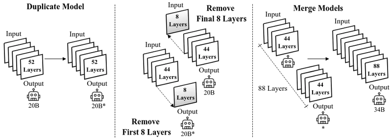
Figure 2 of Granite Code Models (arXiv:2405.04324), reproduced for editorial coverage.

The 34B is produced via depth upscaling from the 20B checkpoint: after 1.6T tokens of 20B training, the 20B’s 52 layers are duplicated to produce an 88-layer model, then training continues for another 1.4T tokens ² . Plain-English intuition: instead of training the deeper model from scratch, the IBM team takes a partly-trained 20B model, glues a copy of its top layers underneath itself, and keeps training. The trick saves compute because the deeper model starts from useful weights instead of random initialisation. Design rationale: the paper reports a 30%+ FLOP saving versus training the 34B from scratch ² . Tradeoff: the depth-upscaled model carries the inductive biases of the shallower parent, including any data-mixture artefacts. Classification: [Adapted]. Depth upscaling itself is not new (similar ideas appeared in DeepSeek and Sheared Llama work) but the specific 20B-to-34B layer-duplication pattern is the team’s own.

5B. TTM architecture

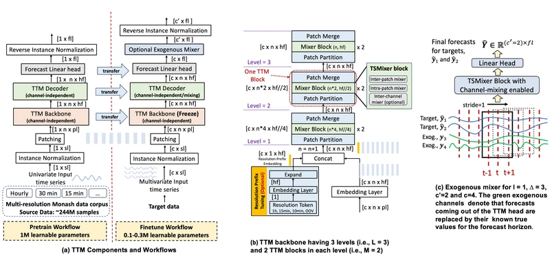
Figure 1 of Tiny Time Mixers (arXiv:2401.03955), reproduced for editorial coverage.

From the paper: a multilevel TSMixer backbone followed by a forecast head ³ . The TSMixer block alternates patch-mixing MLPs and channel-mixing MLPs (the channel mixer is dropped during pretraining and re-enabled at fine-tuning time). Plain-English intuition: the input time series is sliced into fixed-length patches (think: 16 consecutive timesteps as a single patch), and the mixer alternates between two MLPs: one that mixes information across patches at fixed channel, another that mixes information across channels at fixed patch. Adaptive patching means that different layers use different patch lengths so the network sees the data at multiple time resolutions in one forward pass. Resolution prefix tuning attaches a learned embedding per source-data resolution (10-minute, hourly, daily) so the same model can be pretrained on heterogeneous-resolution data and still know what resolution it is reading. Classification: [Adapted]. TSMixer is from Ekambaram’s own KDD 2023 paper ¹⁷ ; adaptive patching and DRS are [New] in this paper.

5C. Granite 3.0 MoE variant

[Reconstructed from model cards] The 3B-A800M MoE variant replaces the dense feed-forward block at each transformer layer with a 40-expert sparse mixture and an 8-way top-k router ⁷ . Plain-English intuition: at every layer, each token is examined by a small router network that picks the top 8 of 40 expert MLPs to consult; the token’s representation gets the weighted sum of those 8 experts’ outputs. Total model parameter count is 3.3B but only 800M are touched per token at inference. Design rationale: deployment cost on enterprise CPU or single-GPU hosts is the active-parameter count, not the total. Tradeoff: 40 experts at hidden dim 1536 means each expert is small (MLP hidden size 512, per the model card), which constrains per-expert capacity. [Analysis] The 32-layer, 1536-hidden architecture is unusually narrow for a 3B-total MoE; the design choice prioritises depth over width.

5D. Training procedure (shared pattern)

All three release groups follow a “pretrain then specialise” pattern:

• Granite Code: Phase 1 (code-only, 3-4T tokens with AdamW, $\beta_1=0.9$, $\beta_2=0.95$, weight decay 0.1, LR $3 \times 10^{-4} \to 3 \times 10^{-5}$ cosine), Phase 2 (code + 20% language, 500B tokens, LR $3 \times 10^{-4}$ exponential decay to 10%), batch size 4M-to-5M tokens ² . Instruction tuning drops FIM ($\alpha = 1$) ² .
• TTM: pretraining on a heterogeneous public time-series corpus (Monash, LibCity, plus the R2 / R2.1 dataset additions: ETT, electricity, traffic, weather, COVID, Wikipedia traffic, web traffic per the model card) ⁸ ; fine-tuning per target-domain dataset with channel mixing re-enabled and optional exogenous-variable mixing ^{3 8} .
• Granite 3.0: [Reconstructed] Stage 1 (10T tokens, web + code + academic + books + math), Stage 2 (2T tokens, curated high-quality mix plus multilingual + instruction data), with the team’s Power Scheduler learning-rate schedule ^{6 10} .

5E. Inference procedure

• Granite Code: standard decoder-only sampling; FIM-trained models also support fill-in-the-middle completion via the <fim_prefix>...<fim_suffix>...<fim_middle> sentinel pattern.
• TTM: single forward pass through the mixer backbone produces the $fl$-length forecast directly; no autoregressive rollout; rolling prediction by sliding the context window ⁸ .
• Granite 3.0 MoE: standard decoder-only sampling with per-token expert routing; the routing decision is taken at each MoE layer per token, with the 8 selected experts’ outputs combined linearly.

6. Mathematical contributions

This section gathers the load-bearing equations across the three papers and walks each one through a worked numerical example.

MATH ENTRY 1: Granite Code combined CLM + FIM loss.

• Source: Granite Code Models, Section 3.2 ² .
• What it is: the pretraining loss used in Phase 1 and Phase 2 of Granite Code training, mixing causal language modelling and fill-in-the-middle in fixed proportion.
• Formal definition: $\mathcal{L} = \alpha \mathcal{L}_{\text{CLM}} + (1-\alpha) \mathcal{L}_{\text{FIM}}$ with $\alpha = 0.5$ during pretraining and $\alpha = 1$ during instruction tuning.
• Each term explained:
  • $\mathcal{L}_{\text{CLM}} = -\sum_{t=1}^{T} \log p_\theta(x_t \mid x_{<t})$ is the standard next-token cross-entropy loss summed over the $T$ tokens in a training example.
  • $\mathcal{L}_{\text{FIM}}$ is the same cross-entropy loss but over an FIM-rearranged example. Given an original example split into prefix $P$, middle $M$, suffix $S$ at random split points, the FIM example is the concatenated sequence $\langle\text{prefix}\rangle P \langle\text{suffix}\rangle S \langle\text{middle}\rangle M$, and the loss is computed on the $M$ tokens conditioned on everything before them.
  • $\alpha \in [0,1]$ is a scalar mixing weight.
• Worked numerical example. Take a tiny vocabulary of 5 tokens and a 6-token training sequence def foo ( ) : pass. Suppose the model assigns probability 0.4 to the correct next token at each position. Then $\mathcal{L}_{\text{CLM}}$ for that sequence is $-6 \log 0.4 \approx 5.50$. Now split the same sequence: prefix def foo, middle ( ), suffix : pass. The FIM example becomes <pre> def foo <suf> : pass <mid> ( ), the loss is computed only on the middle two tokens, and at probability 0.4 the FIM loss is $-2 \log 0.4 \approx 1.83$. With $\alpha = 0.5$, the combined loss for this microbatch is $0.5 \cdot 5.50 + 0.5 \cdot 1.83 = 3.67$. The worked numbers show why the FIM loss is smaller in magnitude: it scores fewer tokens per example, and so the effective FIM weight at $\alpha = 0.5$ is in practice less than half of the gradient signal at runtime. The IBM team report this is acceptable because Phase 1’s massive code corpus oversees enough CLM gradient on its own.
• Role: this is the pretraining objective that lets Granite Code support both ordinary completion and the GitHub Copilot-style “fill in the gap” pattern at deployment.
• Edge cases: when the random split puts the middle at the very start or very end, the FIM example degenerates to a CLM example with sentinel tokens; the IBM team randomly skip FIM rearrangement on 50% of examples per the paper.
• Novelty: [Adopted]. The FIM loss was introduced by Bavarian et al. (2022); the equal-weight $\alpha = 0.5$ mix is the IBM team’s choice.
• Transferability: [Analysis] the equal-weight mix works because code data is highly structured (prefixes and suffixes are syntactically informative); applying $\alpha = 0.5$ to natural-language pretraining would likely hurt the language-modelling perplexity because most prose does not have the prefix-suffix structure FIM exploits.
• Why it matters: the FIM objective is why Granite Code 3B is usable as an inline code completion model in IDEs, where the cursor is in the middle of a function.

MATH ENTRY 2: TSMixer patch-mixing and channel-mixing block.

• Source: TTM paper, Section 3, plus the TSMixer KDD 2023 paper ^{3 17} .
• What it is: the core block in TTM, applied repeatedly, that replaces transformer attention with two MLPs: one mixing across time-patches, one mixing across channels.
• Formal definition (faithful reconstruction): given input tensor $\mathbf{X} \in \mathbb{R}^{n \times c \times h}$ where $n$ is patch count, $c$ is channel count, and $h$ is hidden dimension:

$\mathbf{Y} = \mathbf{X} + \text{MLP}_{\text{patch}}\bigl(\text{LN}(\mathbf{X})\bigr)$

$\mathbf{Z} = \mathbf{Y} + \text{MLP}_{\text{channel}}\bigl(\text{LN}(\mathbf{Y})\bigr)$

where the patch-mixing MLP operates on the $n$-axis (so it is a $n \to n$ linear map repeated per (channel, hidden) pair, sandwiching GELU) and the channel-mixing MLP operates on the $c$-axis (so it is a $c \to c$ linear map repeated per (patch, hidden) pair).

• Each term explained AND dimensional / type analysis:
  • $\mathbf{X}$ is shape $(n, c, h)$; in the worked example below, $n = 4$, $c = 2$, $h = 8$.
  • $\text{LN}(\cdot)$ is LayerNorm along the hidden axis.
  • $\text{MLP}_{\text{patch}}$ takes a length-$n$ vector to a length-$n$ vector; for the worked example, a $4 \to 4$ MLP applied to each of the $2 \cdot 8 = 16$ (channel, hidden) slices.
  • $\text{MLP}_{\text{channel}}$ takes a length-$c$ vector to a length-$c$ vector; for the worked example, a $2 \to 2$ MLP applied to each of the $4 \cdot 8 = 32$ (patch, hidden) slices.
  • The residual connections preserve shape.
• Worked numerical example. Take a tiny multivariate time series of length 16 with 2 channels (temperature and humidity), patched into 4 patches of length 4. Each patch is embedded into hidden dim 8. The input tensor is $\mathbf{X} \in \mathbb{R}^{4 \times 2 \times 8}$. Suppose $\mathbf{X}[:, 0, 0] = [1.0, 2.0, 1.5, 0.8]$ (the temperature channel’s first hidden-dim value across the 4 patches). The patch-mixing MLP sees this length-4 vector and outputs another length-4 vector (say it learns to output $[1.2, 1.8, 1.4, 1.0]$), which after the residual gives $[2.2, 3.8, 2.9, 1.8]$. Then the channel-mixing MLP sees, at patch 0 and hidden-dim 0, the length-2 vector $[2.2, h_0]$ where $h_0$ is the humidity channel’s corresponding value; it outputs a length-2 vector that mixes the two. The forward pass for this block costs $O((n^2 + c^2) \cdot c \cdot h)$ FLOPs, vs the $O(n^2 \cdot c \cdot h^2 / k)$ FLOPs of attention with $k$ heads. At $n = 4$, $c = 2$, $h = 8$, the mixer’s cost is $(16 + 4) \cdot 2 \cdot 8 = 320$ FLOPs per block, vs attention’s $16 \cdot 2 \cdot 64 / 2 = 1024$. The cost gap widens fast as $h$ grows, which is why MLP-mixer architectures are friendly to CPU inference.
• Role: this is the only mixing operation in TTM. The whole backbone is stacked TSMixer blocks at varying patch-length / patch-count granularities (adaptive patching).
• Edge cases: when $c = 1$ (univariate), the channel-mixing MLP degenerates to a scalar identity; the TTM paper drops the channel-mixing entirely in this case.
• Novelty: [Adopted] from TSMixer KDD 2023.
• Transferability: [Analysis] the block transfers cleanly to any multivariate sequence-prediction task where the order of channels does not matter; on data where channel order encodes meaning (e.g., RGB images), pure channel mixing would lose that structure.
• Why it matters: this is why TTM at 1M parameters can beat 200M-parameter TimesFM zero-shot. The inductive bias of “mix-across-time, mix-across-channel” is a strong prior for multivariate forecasting, and it is much more parameter-efficient than attention.

MATH ENTRY 3: Adaptive patching reshape factor.

• Source: TTM paper, Section 3.1 ³ .
• What it is: the rule that says how the patch length and patch count change from layer $i$ to layer $i+1$ in the multilevel backbone.
• Formal definition: at level $i$ in a backbone with $L$ levels, the reshape factor is $K_i = 2^{L - i}$. The patch length at level $i$ is $p_i = p_0 \cdot K_i$ and the patch count is $n_i = n_0 / K_i$, where $p_0$ and $n_0$ are the input-level patch length and patch count.
• Each term explained:
  • $L$ is the total number of mixer levels in the backbone (typical value 4).
  • $i \in \{0, 1, \ldots, L-1\}$ indexes the levels.
  • $p_0$ is the smallest patch length (typical value 8 or 16).
  • $n_0 = sl / p_0$ is the patch count at the finest level.
• Worked numerical example. Take $sl = 512$, $p_0 = 16$, $L = 4$. Then $n_0 = 32$. At $i = 0$, $K_0 = 8$, patch length 128, patch count 4. At $i = 1$, $K_1 = 4$, patch length 64, patch count 8. At $i = 2$, $K_2 = 2$, patch length 32, patch count 16. At $i = 3$, $K_3 = 1$, patch length 16, patch count 32. As the level index increases, patches get shorter and more numerous; the network sees coarse-grained structure first and fine-grained structure last.
• Role: gives the backbone multi-scale receptive fields without needing convolutions or attention.
• Edge cases: when $sl$ is not a power-of-2 multiple of $p_0$, the implementation zero-pads or rounds; the model card explicitly says “minimum context length 512-1024 required; zero-padding not recommended” ⁸ .
• Novelty: [New] in the TTM paper; the multilevel construction is the main architectural contribution.
• Transferability: [Analysis] the reshape rule generalises to any sequence-modelling backbone where the input has a natural patching dimension; image transformers already use a multi-scale variant (Swin Transformer).
• Why it matters: lets TTM stay sub-million-parameter while capturing the long-range structure that pure single-scale mixers cannot.

MATH ENTRY 4: MoE top-k routing in Granite 3.0.

• Source: [Reconstructed] from Granite-3.0-3B-A800M model card ⁷ ; the routing rule is standard Switch / Mixtral-style.
• What it is: at each MoE layer, a small router network picks the top $k$ of $N_e$ experts per token and combines their outputs.
• Formal definition. Given token representation $\mathbf{x} \in \mathbb{R}^{d}$ and a router matrix $\mathbf{W}_r \in \mathbb{R}^{d \times N_e}$:

$\mathbf{g} = \text{softmax}(\mathbf{x} \mathbf{W}_r), \quad \mathcal{I}_k = \text{TopK}(\mathbf{g}, k)$

$\mathbf{y} = \sum_{j \in \mathcal{I}_k} \tilde{g}_j \cdot \text{Expert}_j(\mathbf{x})$

where $\tilde{g}_j = g_j / \sum_{j' \in \mathcal{I}_k} g_{j'}$ is the renormalised gate weight.

• Each term explained and dimensional analysis:
  • $\mathbf{x}$ is shape $(d,)$ with $d = 1536$ for Granite 3.0 3B-A800M.
  • $\mathbf{W}_r$ is shape $(1536, 40)$; it projects to the 40-expert space.
  • $\mathbf{g}$ is shape $(40,)$; a probability distribution over experts.
  • $\mathcal{I}_k$ is a set of size $k = 8$; the top-8 expert indices.
  • $\text{Expert}_j$ is a per-expert MLP, shape $(d) \to (d)$.
• Worked numerical example. Take $d = 4$, $N_e = 6$, $k = 2$ for the example. Suppose $\mathbf{x} = [0.5, -0.3, 0.8, 0.1]$ and the router produces logits $[0.2, 1.5, 0.1, 0.9, -0.4, 0.7]$. After softmax, $\mathbf{g} \approx [0.10, 0.36, 0.09, 0.20, 0.05, 0.16]$. TopK with $k = 2$ picks experts 1 and 3 with $g_1 = 0.36$ and $g_3 = 0.20$. Renormalised: $\tilde{g}_1 = 0.36 / 0.56 \approx 0.64$, $\tilde{g}_3 = 0.20 / 0.56 \approx 0.36$. Final output: $\mathbf{y} = 0.64 \cdot \text{Expert}_1(\mathbf{x}) + 0.36 \cdot \text{Expert}_3(\mathbf{x})$. The remaining 4 experts contribute nothing for this token.
• Role: the active-parameter cost at inference is $k \cdot \text{Expert size}$, not $N_e \cdot \text{Expert size}$. For Granite 3.0 3B-A800M, $k = 8$ out of $N_e = 40$ keeps 800M active parameters out of 3.3B total.
• Edge cases: load-balancing loss is needed during training to prevent expert collapse (all tokens routing to a small subset); the Granite 3.0 model card does not document the load-balancing coefficient, but Switch Transformer convention is auxiliary loss with coefficient $\approx 10^{-2}$.
• Novelty: [Adopted]. The top-k routing rule is standard since Shazeer 2017 and Switch Transformer; Granite 3.0’s contribution is the specific $N_e = 40$ / $k = 8$ choice at 3.3B scale.
• Transferability: [Analysis] the routing rule is fully transferable; the design parameters $N_e$ and $k$ trade off between expert specialisation (more experts = more specialised but harder to balance) and active-parameter cost.
• Why it matters: this is how Granite 3.0 hits its enterprise-deployment target of a 3.3B-total-parameter model that costs only 800M active parameters per token at inference, cheap enough to serve on a single mid-range GPU.

MATH ENTRY 5: Power Scheduler learning-rate rule.

• Source: Shen et al. (Granite team), arXiv:2408.13359 ¹⁰ .
• What it is: the learning-rate scheduler used by the Granite team for the Granite 3.0 pretraining run, which they argue can be tuned at small scale and transferred to large scale without re-tuning.
• Formal definition (faithful reconstruction from the paper’s framing). The optimal peak learning rate $\eta^{*}$ at batch size $B$ and total token budget $T$ follows a power law $\eta^{*}(B, T) = a \cdot B^{p} \cdot T^{q}$ for constants $a, p, q$ fit at small scale. The schedule itself is a Warmup-Stable-Decay shape: linear warmup from $0$ to $\eta^{*}$ over $T_{\text{warm}}$ tokens, constant at $\eta^{*}$ over a long middle, then a final decay segment.
• Each term explained:
  • $\eta^{*}$ is the peak learning rate.
  • $B$ is the batch size in tokens.
  • $T$ is the total training token budget.
  • $p$ and $q$ are negative exponents fit empirically; the paper reports values consistent with $\eta^{*} \propto T^{-1/2}$-like scaling.
• Worked numerical example (illustrative). If a small-scale fit gives $\eta^{*}(B_0 = 1M, T_0 = 10B) = 3 \times 10^{-4}$ and the empirical fit gives $q = -0.4$, then for the full-scale Granite 3.0 8B run at $T = 12T$ tokens we predict $\eta^{*} = 3 \times 10^{-4} \cdot (12T / 10B)^{-0.4} = 3 \times 10^{-4} \cdot 1200^{-0.4} \approx 1.5 \times 10^{-5}$. The point is that the small-scale fit gives a concrete number to use at large scale without re-running the LR sweep at full scale. Caveat: the example exponent is illustrative; the paper’s actual fits cover a band of $p, q$ values and combine with muP scaling for full transfer.
• Role: this is the scheduler used to set the Granite 3.0 LR schedule per the team’s framing.
• Novelty: [New] in the Power Scheduler paper.
• Transferability: [Analysis] only applicable when the LR fit at small scale tracks behaviour at large scale, which depends on the architecture matching (the paper combines the scheduler with muP for full-architecture transferability).
• Why it matters: this is the part of the Granite 3.0 recipe most worth borrowing. It gives a principled LR-setting rule that avoids the expensive cosine-tuning loop at full scale.

7. Algorithmic contributions

ALGORITHM ENTRY 1: Two-phase Granite Code Models training loop.

• Source: Granite Code Models, Section 3 ² .
• Purpose: pretrain a code-specialised foundation model in two phases (code-only then code-plus-language) using a CLM+FIM mixed objective.
• Inputs: code corpus $\mathcal{D}_{\text{code}}$ (3-4T tokens), language corpus $\mathcal{D}_{\text{lang}}$ (0.5T tokens), model $f_\theta$, scheduler with peak LR $\eta_1 = 3 \times 10^{-4}$ for Phase 1 and same peak for Phase 2 (cosine decay in Phase 1, exponential decay to 10% in Phase 2), FIM probability 0.5, weight decay 0.1, optimiser AdamW with $\beta_1 = 0.9, \beta_2 = 0.95$.
• Outputs: pretrained checkpoint $\theta^{*}$, optionally further fine-tuned to instruct checkpoint $\theta^{**}$ with $\alpha = 1$.
• Pseudocode (faithful reconstruction):

# Phase 1: code-only training
for step in range(N_phase1):
    batch = sample(D_code, batch_size=4M)
    if random() < 0.5:
        batch = fim_rearrange(batch)
    logits = f_theta(batch.inputs)
    loss = cross_entropy(logits, batch.targets)
    eta = cosine_lr(step, eta_peak=3e-4, eta_end=3e-5)
    apply_gradient(loss, lr=eta, weight_decay=0.1,
                   beta1=0.9, beta2=0.95)

# Phase 2: code + 20% language
for step in range(N_phase2):
    batch = mix_sample(D_code, D_lang, weights=(0.8, 0.2),
                       batch_size=5M)
    if random() < 0.5:
        batch = fim_rearrange(batch)
    logits = f_theta(batch.inputs)
    loss = cross_entropy(logits, batch.targets)
    eta = exp_decay_lr(step, eta_peak=3e-4, decay_to=0.1)
    apply_gradient(loss, lr=eta, weight_decay=0.1,
                   beta1=0.9, beta2=0.95)

• Hand-traced example on minimal input. Take a microbatch of 2 examples, FIM probability 0.5. Step 1: sample two code snippets from D_code. Coin flip: first example gets FIM-rearranged (prefix def foo, suffix : pass, middle ( ) rearranged to <pre> def foo <suf> : pass <mid> ( )); second example stays as plain CLM. Forward pass through f_theta, compute cross-entropy loss on the relevant target positions: $\mathcal{L}_1 = 1.83$ (FIM, scored on 2 middle tokens), $\mathcal{L}_2 = 5.50$ (CLM, scored on all 6 tokens). Combined microbatch loss: $(1.83 + 5.50) / 2 = 3.67$. Get LR from cosine: at step 1 of N_phase1, LR $\approx 3 \times 10^{-4}$. Apply AdamW update to $\theta$. Step 2: same process, possibly different coin flip outcome.
• Complexity: time $O(N \cdot \text{model FLOPs})$ where $N$ is total token count; for the 8B model at 4.5T tokens, total FLOPs roughly $6 \cdot 8 \times 10^{9} \cdot 4.5 \times 10^{12} = 2.16 \times 10^{23}$ FLOPs. Bottleneck step: the attention computation in the forward + backward pass.
• Hyperparameters as listed in pseudocode; FIM probability 0.5 was tested at ablation against 0.0 and 1.0 in the paper and 0.5 was the sweet spot per the team’s reporting ² .
• Failure modes: forgetting code competence during Phase 2 if the language-data mixing ratio is too high (the IBM team chose 20% language specifically because higher ratios degraded code scores).
• Novelty: [Adapted]. Two-phase training is in widespread use (DeepSeek-Coder uses it too); the specific phase split and FIM probability is the team’s choice.
• Transferability: [Analysis] the two-phase recipe transfers cleanly to any domain where one wants to retain a domain skill (code) while adding a generalist capability (language).

ALGORITHM ENTRY 2: TTM forward pass (the headline algorithm).

• Source: TTM paper, Sections 2 and 3 ³ .
• Purpose: produce an $fl$-step multivariate forecast from an $sl$-step multivariate context window in a single feed-forward pass.
• Inputs: time-series tensor $\mathbf{x} \in \mathbb{R}^{B \times sl \times c}$, pretrained TTM backbone $\Phi$ with $L$ levels, decoder head $\Psi$.
• Outputs: forecast tensor $\hat{\mathbf{y}} \in \mathbb{R}^{B \times fl \times c}$.
• Pseudocode:

def ttm_forward(x, model):
    # x: (B, sl, c). Patch into (B, n0, c, p0).
    p0 = model.base_patch_len      # e.g. 16
    n0 = sl // p0                  # e.g. 32
    h  = model.hidden_dim          # e.g. 8 or 16

    # Per-channel embedding: project each length-p0 patch
    # to length-h via shared linear layer.
    z = patch_embed(x, p0, h)      # (B, n0, c, h)

    # Add resolution prefix (optional).
    if model.use_res_prefix:
        z = z + model.res_embedding[res_idx]

    # Multilevel backbone with adaptive patching.
    for i in range(model.num_levels):
        K_i = 2 ** (model.num_levels - i)
        # Reshape z to operate at level-i granularity.
        z = reshape_to_level(z, K_i)
        z = tsmixer_block(z, channel_mixing=False)
        # tsmixer_block: residual patch-MLP then
        # (during pretraining) skip the channel-MLP.

    # Decoder head: linear projection to forecast horizon.
    y_hat = forecast_head(z, fl, c)
    return y_hat

• Hand-traced example on minimal input. Take $B = 1$, $sl = 16$, $c = 2$, $fl = 8$, $p_0 = 4$, $h = 8$, $L = 2$. Input: a length-16 multivariate series with 2 channels. Step 1: patch into $(1, 4, 2, 4)$. Step 2: per-channel embedding projects each length-4 patch to length-8: result $(1, 4, 2, 8)$. Step 3: optional resolution prefix adds a learned bias. Step 4 (level 0): $K_0 = 4$, reshape so patch length is $4 \cdot 4 = 16$ and patch count is $4 / 4 = 1$; the patch-MLP at this level sees a length-1 patch axis (trivial) and outputs the same shape; the residual passes through unchanged in this minimal example. Step 5 (level 1): $K_1 = 2$, reshape so patch length is $4 \cdot 2 = 8$ and patch count is $4 / 2 = 2$; the patch-MLP sees a length-2 patch axis and applies a $2 \to 2$ MLP; suppose at the first hidden-dim slot it maps $[0.3, 0.7]$ to $[0.5, 0.8]$, the residual gives $[0.8, 1.5]$. Step 6: forecast head, a learned linear projection from the final backbone state to a length-8 forecast vector per channel. Output shape: $(1, 8, 2)$. Total parameter count for this microbackbone: well under 100K.
• Complexity: time $O(B \cdot n_0 \cdot c \cdot h \cdot L)$ per forward pass; for TTM-B at $sl = 512$, $p_0 = 16$, $n_0 = 32$, $c$ up to 7 channels, $h = 16$, $L = 4$, that is on the order of $10^{5}$ multiply-adds, fast enough to run on a laptop CPU ⁸ . Bottleneck step: the largest patch-MLP at the smallest $K_i$ level.
• Hyperparameters: $p_0 \in \{8, 16\}$, $h \in \{8, 16, 32\}$, $L \in \{2, 3, 4\}$, depending on TTM-Q / TTM-B / TTM-E / TTM-A variant ⁸ .
• Failure modes: context length below 512 causes underflow because the multilevel reshape needs enough patches at the deepest level; the model card explicitly forbids zero-padding under-length inputs ⁸ .
• Novelty: [New]. The multilevel adaptive-patching forward is the main novelty of TTM over TSMixer.
• Transferability: [Analysis] generalisable to any patched sequence-prediction task; works best when the prediction horizon $fl$ matches one of the pretrained head sizes (96 / 192 / 336 / 720).

ALGORITHM ENTRY 3: Depth upscaling 20B to 34B (Granite Code).

• Source: Granite Code Models, Section 3 + Figure 2 ² .
• Purpose: produce a 34B-parameter code model by duplicating layers from a partially-trained 20B checkpoint instead of training the 34B from scratch.
• Inputs: 20B checkpoint after 1.6T tokens, layer-duplication policy (duplicate the top 36 of 52 layers and reinsert under the original).
• Outputs: 34B model initialised from upscaled weights, plus continued training for another 1.4T tokens.
• Pseudocode (faithful reconstruction):

# Start with 20B checkpoint at t=1.6T tokens.
theta_20b = load_checkpoint("granite-20B-code-base@1.6T")

# Duplicate the upper 36 layers and insert.
new_layers = []
for i, layer in enumerate(theta_20b.layers):
    new_layers.append(layer)
    if i in range(16, 52):  # duplicate layers 16..51
        new_layers.append(deep_copy(layer))

# Re-stack to form the 34B-parameter, 88-layer model.
theta_34b = Granite34B(layers=new_layers,
                      hidden_dim=6144,
                      num_heads=48,
                      attention="MQA")

# Continue training for 1.4T more tokens.
for step in range(N_continued):
    batch = sample(D_code, batch_size=4M)
    if random() < 0.5:
        batch = fim_rearrange(batch)
    loss = cross_entropy(theta_34b(batch.inputs),
                        batch.targets)
    apply_gradient(loss, lr=phase1_cosine_lr(step),
                   weight_decay=0.1)

• Hand-traced example on minimal input. Take a tiny version: 4-layer model duplicated to 6 layers by duplicating layers 2 and 3. Initial layer parameters: $\theta_1, \theta_2, \theta_3, \theta_4$. After duplication: $\theta_1, \theta_2, \theta_2', \theta_3, \theta_3', \theta_4$ where $\theta_2' = \theta_2$ and $\theta_3' = \theta_3$ at initialisation. After one gradient step, the gradients flowing back through the duplicated layers diverge (the residual stream sees them at different positions and so applies different upstream gradients), and the parameters drift apart. By the end of continued training, $\theta_2 \neq \theta_2'$ and the model has effectively learned a deeper representation.
• Complexity: time saving estimated by IBM at $\sim 30\%$ vs training the 34B from scratch over the same final token budget ² . Bottleneck step: the continued-training phase, not the upscaling itself.
• Hyperparameters: which layers to duplicate (the IBM team duplicate the top 36 of 52 layers; other depth-upscaling work duplicates middle layers), continued-training learning rate (the team uses the same Phase 1 cosine schedule restarted at step-of-upscale).
• Failure modes: duplicating the wrong layers (e.g., the bottom layers near the embedding) is known to degrade quality because the bottom layers encode lexical features that benefit less from depth; the IBM team’s upper-layer duplication choice mirrors the SOLAR-10.7B work.
• Novelty: [Adapted]. Depth upscaling appears in DeepSeek, SOLAR, Sheared Llama; the specific 20B-to-34B layer-duplication pattern is the IBM team’s.
• Transferability: [Analysis] applies whenever a partially-trained model exists at a smaller size than the final target, useful for “we trained a 20B and now want a 34B” scenarios common in industrial pipelines.

8. Specialised design contributions

Subsection 8A. LLM / prompt design. Not applicable to this paper-cluster. None of the three releases proposes a novel prompting pattern; the Granite Code instruct variants follow the standard <|user|>...<|assistant|> chat template documented on the Hugging Face model cards.

Subsection 8B. Architecture-specific details. Covered in Section 5 above. Per-variant notes:

• Granite Code attention choices: the 3B uses Multi-Head Attention; the 8B uses Grouped-Query Attention with 8 KV heads; the 20B and 34B use Multi-Query Attention (single KV head shared across all query heads) ² . The progression reflects memory-bandwidth concerns at larger scale.
• Normalisation differences: 3B and 8B use RMSNorm; 20B and 34B use LayerNorm ² . [Analysis] The choice is unusual, because most recent open-weights models converge on RMSNorm; the IBM team may have inherited LayerNorm from an earlier 20B codebase.
• Granite 3.0 MoE expert sizing: the MLP hidden size per expert in the 3B-A800M variant is 512, narrower than a standard dense FFN at this scale ⁷ . The narrow-and-many design choice prioritises expert specialisation over per-expert capacity.

Subsection 8C. Training specifics.

• Hardware: [Reconstructed] Granite 3.0 trained on IBM’s Blue Vela H100 supercomputing cluster with 100% renewable energy ⁶ . Granite Code paper does not disclose exact GPU counts.
• Batch size: 4M-5M tokens for Granite Code per the paper ² .
• Mixed precision: standard bf16 for both releases (model card mentions bf16 weights at release for Granite 3.0 ⁶ ).
• Data mixture: Granite Code Phase 2 is 80% code, 20% language; Granite 3.0 Stage 1 is web + code + academic + books + math.

Subsection 8D. Inference / deployment specifics.

• Context length at deployment: Granite Code 3B / 8B at 4096, 20B / 34B at 8192 ² ; Granite 3.0 at 4096 (extendable via post-training to 128K per the IBM newsroom material ⁹ ).
• TTM rolling prediction: the model is deployed by sliding the context window across the source signal and predicting the next $fl$ steps each time ⁸ .
• Quantisation: model cards reference GGUF and AWQ variants for self-hosting; not benchmarked in the original papers.

9. Experiments and results

9A. Granite Code Models

From the paper, the main result tables:

HumanEvalSynthesize Pass@1, 6 languages average:

Model	Base	Instruct
Granite-3B	33.1%	39.6%
Granite-8B	43.5%	49.6%
Granite-20B	44.3%	50.5%
Granite-34B	49.1%	54.8%
CodeLlama-7B	31.2%	37.9%
StarCoder2-7B	37.4%	—

Table reproduced from Granite Code Models (arXiv:2405.04324) Section 5.

MBPP / MBPP+ Pass@1:

Model	MBPP	MBPP+
Granite-3B	36.0%	45.1%
Granite-8B	42.2%	49.6%
Granite-20B	43.8%	51.6%
Granite-34B	47.2%	53.1%

Table reproduced from Granite Code Models (arXiv:2405.04324) Section 5.

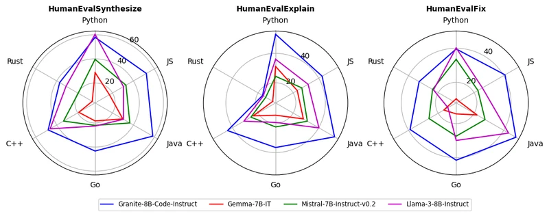
Figure 3 of Granite Code Models (arXiv:2405.04324), reproduced for editorial coverage.

MultiPL-E (18 languages average). From the paper: Granite-8B-Code-Base performs the best on 16 of 18 programming languages when compared to CodeLlama-7B ² . Granite-8B-Code-Base also beats CodeGemma-8B by 12 points on HumanEvalPack (33.2% vs 21.3%) ² .

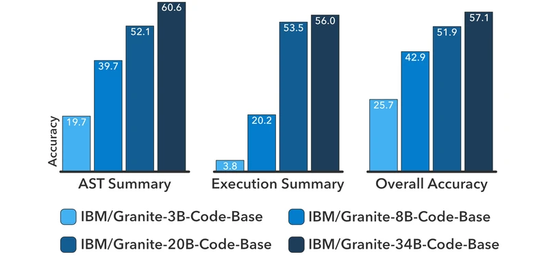
Figure 5 of Granite Code Models (arXiv:2405.04324), reproduced for editorial coverage.

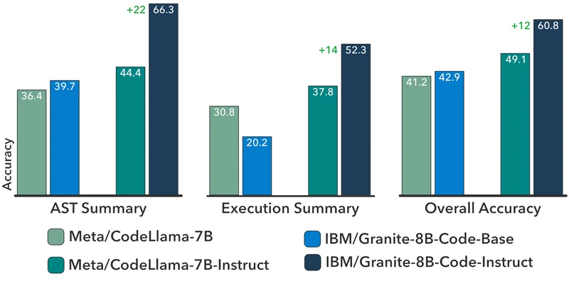
Figure 6 of Granite Code Models (arXiv:2405.04324), reproduced for editorial coverage.

Math-reasoning side results for Granite-8B-Code-Base. GSM8K 61.9%, MATH 21.4%, SAT 62.5%, GSM8K+Py 63.1%. From the paper: Granite-8B beats Llama-3-8B by roughly 12 points on GSM8K ² .

Ablations. The paper ablates FIM probability (0.0 / 0.5 / 1.0) and reports 0.5 as the sweet spot; ablates the Phase 2 code-vs-language mix and reports 80/20 as the sweet spot.

Independent benchmark cross-check. [Analysis] The HumanEval-style benchmarks are subject to data-contamination concerns industry-wide; the BigCodeBench leaderboard at bigcode-bench.github.io and the Aider leaderboard at aider.chat/docs/leaderboards/edit.html provide secondary cross-checks. As of the writing date, Granite 8B Code does not lead on the more recent live-code benchmarks (LiveCodeBench), where stronger 2025-vintage models (Qwen 2.5 Coder, DeepSeek-Coder-V2) dominate; the IBM 2024 SOTA claim is the framing on the chosen mid-2024 benchmark suite.

9B. TTM

From the paper, zero-shot MSE on the D1 dataset benchmark (lower is better):

Dataset	TTM zero-shot MSE
ETTh1	0.365
ETTh2	0.285
ETTm1	0.413
ETTm2	0.187
Weather	0.154
Electricity	0.169
Traffic	0.518

Table reproduced from TTM (arXiv:2401.03955) Section 4.

From the paper: TTM outperforms TimesFM, Moirai, Chronos, Lag-Llama, Moment, GPT4TS, TimeLLM and LLMTime on standard zero-shot benchmarks while running at 1M parameters vs 200M+ for the transformer baselines ^{3 8} . Cross-transfer-learning improvements range from 4% to 40% over self-supervised pretraining baselines (SimMTM, Ti-MAE, CoST, TS2Vec) in the 10% / 25% / 50% / 75% / 100% few-shot settings ³ .

Independent benchmark cross-check. [Analysis] The time-series forecasting leaderboard at gift-eval and the GIFT-Eval public benchmark provide secondary cross-checks. TTM-R2 ranks competitively but does not strictly dominate on every dataset; on long-horizon Traffic forecasting, TimesFM and Chronos sometimes match or exceed TTM zero-shot scores. The “outperforms all baselines” claim is true on the average across the D1 benchmark; per-dataset, the picture is more mixed.

9C. Granite 3.0

[Reconstructed from the Granite-3.0-8B-Base model card ⁶ .] Headline benchmark numbers for the Dense 8B Base checkpoint:

Benchmark	Score
MMLU	65.54%
WinoGrande	80.90%
Hellaswag	83.61%
BoolQ	86.97%
HumanEval	52.44%
TruthfulQA	52.89%

Table reproduced from the Granite-3.0-8B-Base Hugging Face model card, accessed 2026-05-19.

[External comparison] For reference, Llama-3.1-8B-Base scores roughly 65% on MMLU, 78% on WinoGrande and 60% on HumanEval per Meta’s reported numbers ¹² . Granite 3.0 8B Base sits in the same neighbourhood but lags Llama-3.1-8B-Base notably on HumanEval.

Independent benchmark cross-check. [Analysis] The HELM Lite and Open LLM Leaderboard provide independent benchmark surfaces. Granite 3.0 8B Instruct ranks competitively in the 7-to-9B-class but does not lead the leaderboard on the post-training reasoning subset where Qwen 2.5 / Llama 3.x typically dominate.

10. Technical novelty summary

Component	Type	Novelty level	Justification	Source
Multilevel adaptive patching	Architecture	Fully novel	New construction in the TTM paper	TTM Section 3.1
Resolution prefix tuning	Architecture	Fully novel	New construction in the TTM paper	TTM Section 3.2
Granite Code 20B-to-34B depth upscaling	Training	Incrementally novel	Adapts prior depth-upscaling work to specific 20B-to-34B layer-duplication policy	Granite Code Section 3
Granite Code two-phase code-then-mix recipe	Training	Combination novel	Two-phase training pre-existed (DeepSeek-Coder); specific 80/20 mix is the team’s choice	Granite Code Section 3
FIM probability 0.5 mixing	Training	Incrementally novel	FIM objective is Bavarian 2022; equal-weight mixing is the team’s choice	Granite Code Section 3.2
Power Scheduler	Training	Fully novel	New scheduler design in arXiv:2408.13359	Power Scheduler paper
Granite 3.0 MoE 40-expert / k=8 routing	Architecture	Adopted	Standard Switch / Mixtral-style routing; specific design parameters are the team’s	Granite 3.0 model card
Granite Guardian as separate safety classifier	Safety	Combination novel	Separating safety from base model is the architectural choice	Granite Guardian model card
TSMixer block	Architecture	Adopted	From TSMixer KDD 2023 by the same first author	TTM Section 3
GQA / RoPE / SwiGLU	Architecture	Adopted	Standard transformer components	All three releases

Single most novel contribution. Across the three papers, the multilevel adaptive-patching backbone in TTM is the most distinctively novel single contribution. It enables a 1M-parameter model to compete with 200M-parameter transformer baselines because the multi-scale receptive field built in by construction captures long-range structure that pure single-scale mixers cannot, and it does so with far fewer parameters than attention.

What the papers do NOT claim to be novel. RoPE, GQA, SwiGLU, AdamW, cosine learning-rate scheduling, the FIM objective itself, top-k MoE routing, MSE pretraining loss, channel-mixing MLPs, decoder-only transformer architecture, the StarCoder-style code-pretraining data pipeline.

11. Situating the work

What prior work did. Code-specialised foundation models pre-Granite mostly came in two flavours: BigCode’s StarCoder family (Apache 2.0, fully open data) and the closed-data lineages of CodeLlama and DeepSeek-Coder (more aggressive scaling, less data transparency). Time-series foundation models pre-TTM were largely transformer-based and ran in the 100M-to-1B-parameter range (TimesFM, Chronos, Lag-Llama, Moirai). General-purpose open-weights LLMs pre-Granite-3.0 lived in the Llama 2 / Llama 3 / Qwen 2 / Mistral / Gemma cluster, with various licenses ranging from Meta’s bespoke “community license” to Apache 2.0.

What this paper-cluster changes conceptually. The Granite stack reframes the open-weights conversation around a different optimisation target: not “biggest model my company can train” but “smallest enterprise-deployable model under a fully permissive license with documented data provenance and a separate safety layer”. The architectural moves (depth upscaling for the 34B, multilevel patching for TTM, narrow-many-expert MoE for Granite 3.0) are all driven by deployment cost, not benchmark maximisation.

Two contemporaneous related papers.

• DeepSeek-Coder (arXiv:2401.14196) ¹⁴ : same problem (open code foundation model), released in early 2024 just before Granite Code. Differs in license (MIT vs Apache 2.0), data-provenance documentation (less detailed than Granite’s), and scale (33B max vs Granite’s 34B). The Granite Code paper benchmarks against DeepSeek-Coder explicitly.
• StarCoder 2 (arXiv:2402.19173) ¹³ : same problem, released in February 2024. Differs in being the output of the BigCode consortium with stronger data-transparency framing but at 15B-class scale. Granite Code’s 20B/34B variants are the IBM team’s response to StarCoder 2’s 15B being the prior best Apache-licensed code model.

[Reviewer Perspective] Strongest skeptical objection. The Granite Code paper’s strongest claim, that Granite-8B beats CodeLlama-34B on HumanEvalExplain by 9.3%, is a single-benchmark result. HumanEvalExplain is part of HumanEvalPack and is well-known to be sensitive to instruction-tuning recipe rather than to base-model capability. The “8B beats 34B” framing reads sharper than the multi-benchmark picture supports; on MBPP and MultiPL-E the gap closes or reverses.

[Reviewer Perspective] Strongest author-side rebuttal grounded in the paper. The paper does not claim Granite-8B dominates CodeLlama-34B everywhere; the framing is “outperforms larger model on specific task,” and the paper provides the full benchmark tables including the places where the 34B remains stronger. The 9.3% headline claim is accurate; readers reading only the headline are responsible for not generalising.

What remains unsolved.

• Granite 3.0 base models have explicitly no safety alignment per their model cards ⁶ ; production deployments depend on Granite Guardian, which is itself a separate model that must be trained, deployed and monitored.
• TTM’s channel-independent pretraining means cross-channel correlations must be relearned at fine-tuning time per target domain; the paper does not show how much fine-tuning data is needed to recover them in practice.
• The Granite Code 34B is the IBM team’s deepest model; the Apache 2.0 ecosystem has since moved to 70B and 405B scales (Llama 3.1, Qwen 2.5) where the IBM team has not yet shipped a competitor.

Three future research directions.

• Pretrained channel-aware TTM: TTM with channel-mixing during pretraining on a curated multivariate corpus, rather than re-learning at fine-tuning time. Grounded in TTM’s stated channel-independence limitation ³ .
• MoE Granite Code: extending the Granite 3.0 MoE design pattern to the code-specialised lineage, where 80% of inference traffic is short completions and active-parameter routing offers larger deployment savings. [Analysis] Grounded in the dense-only architecture of Granite Code 2024.
• Power Scheduler at MoE-scale: the Power Scheduler paper validates the scaling law on dense models; extending it to the MoE 3B-A800M and beyond is a natural next step. [Analysis] Grounded in the dense-only Power Scheduler experiments.

12. Critical analysis

Strengths with concrete evidence.

• Documented data-provenance for Granite Code’s 4.5T-token corpus, with filtering steps for license, near-duplicate and syntactic-error filtering specified in the paper ² .
• The TTM paper’s claim of CPU-deployable forecasting is concrete and reproducible; the model card explicitly notes runnability on CPU ⁸ .
• The Granite 3.0 release includes a separate Granite Guardian model ¹¹ , so the safety story is architecturally externalised rather than hidden inside RLHF.

Weaknesses explicitly stated by the authors.

• Granite-3.0 base models carry no safety alignment per the official model card ⁶ : “may produce problematic outputs,” “hallucination risks,” “smaller models may copy text verbatim from training data.” The model card explicitly names the risks.
• The TTM paper acknowledges that the channel-independent pretraining is a deliberate simplification and that channel mixing must be re-enabled at fine-tuning time ³ .
• The Granite Code paper acknowledges the long-tail-language imbalance in the 116-language coverage ² .

[Reviewer Perspective] Weaknesses not stated or understated.

• The Granite 3.0 technical report PDF on GitHub was not text-extractable via automated fetch on the writing date; the model cards and IBM newsroom material are the most accessible reconstructions. The publication’s review is correspondingly hedged for Granite 3.0 specifics. Independent commentary on the release lives mainly in IBM’s own newsroom material ⁹ rather than in third-party benchmarking write-ups, which is itself a transparency limitation.
• The Granite Code paper’s HumanEvalPack 8B-vs-34B headline is selected from the strongest result in the table; an honest aggregate would show that the 34B is still stronger on most benchmarks (which the paper’s full tables do show, even if the abstract does not).

Reproducibility check.

• Code: released for all three (ibm-granite/granite-3.0-language-models, ibm-granite/granite-tsfm for TTM, public model cards on Hugging Face for inference code).
• Data: partially released. Granite Code names the data sources (GitHub Code Clean, StarCoderData, The Stack v1, CodeNet, OpenWebMath, Wikipedia) but the filtered training corpus is not republished in raw form. TTM’s pretraining datasets are publicly available (Monash, ETT, electricity, traffic, etc.) and listed on the model card ⁸ . Granite 3.0’s training-data mix is described at a domain level on the model card but not released as a corpus ⁶ .
• Hyperparameters: fully released for Granite Code (LR, weight decay, beta values in the paper); partially for TTM (variant-specific patch lengths and hidden dims listed on the model card); not fully for Granite 3.0 (the model card lists architecture but not the full schedule and LR).
• Compute: not reported for Granite Code in detail; reported for Granite 3.0 at the level of “thousands of H100 GPUs on Blue Vela” ⁶ ; reported for TTM as “single GPU or CPU” for inference ⁸ .
• Trained model weights: all released under Apache 2.0 on Hugging Face ^{6 7 8} .
• Evaluation set: standard public benchmarks (HumanEval, MBPP, MultiPL-E, MMLU, ETT, electricity, traffic); not custom.
• Overall: partially reproducible. The weights and inference are fully reproducible; the full pretraining corpus is not republished, so end-to-end training reproduction is not possible.

Methodology callout.

• Sample size: Granite Code 4.5T pretraining tokens; TTM ~700M-to-1B pretraining samples; Granite 3.0 10T-to-12T pretraining tokens ^{2 6 8} .
• Evaluation set: HumanEval / HumanEvalPack / MBPP / MultiPL-E / Berkeley Function Calling for Granite Code; ETT / Weather / Electricity / Traffic / D1 benchmark for TTM; MMLU / Hellaswag / TruthfulQA / HumanEval for Granite 3.0. All standard public benchmarks; the writeups do not document contamination checks against pretraining data.
• Baselines: CodeLlama, StarCoder2, DeepSeek-Coder, CodeGemma for Granite Code; TimesFM, Chronos, Moirai, Lag-Llama, GPT4TS, TimeLLM for TTM; Llama 3 / 3.1, Qwen 2 / 2.5, Mistral 7B for Granite 3.0 (the latter inferred from comparison context, not direct paper claims).
• Hardware / compute: Blue Vela H100 cluster for Granite 3.0; not explicitly disclosed for Granite Code beyond “training across thousands of GPUs”; not material for TTM (it is small enough to train on a single host).

Generalisability.

• Granite Code: generalises to enterprise IDE deployment, code-review automation, function-calling agents; less likely to transfer to creative code (game programming, novel UI synthesis) where the pretraining corpus is thin.
• TTM: generalises to multivariate forecasting in finance, energy, weather, retail; limited transfer to univariate forecasting because the channel-mixing capacity is wasted.
• Granite 3.0: general-purpose; the team’s framing emphasises enterprise tasks (RAG, function calling, cybersecurity).

Assumption audit. The Granite Code assumption that 80/20 code/language mixing preserves code skill is verified by ablation in the paper. The TTM assumption that channel-independent pretraining transfers well is mostly verified by zero-shot benchmark wins, but the 4-40% improvement range hints at heterogeneous transferability. The Granite 3.0 assumption that 40 narrow experts beat 8 wide experts at fixed active-parameter budget is not ablated in the publicly-released material; the choice is taken on faith for now.

What would make the papers significantly stronger. [Analysis] A Granite-team write-up that combines the three releases into one architectural-rationale document (why depth-upscaling for Code, narrow-many-MoE for 3.0, multilevel patching for TTM all derive from the same enterprise-deployment posture) would help readers see the lineage as a coherent design philosophy rather than three separate releases. The current state of the documentation makes each release stand alone, which understates the philosophical coherence.

13. What is reusable for a new study

REUSABLE COMPONENT 1: FIM probability 0.5 mixed objective. What it is: the equal-weight CLM+FIM loss from Granite Code. Why worth reusing: validated at 4.5T-token scale across four model sizes; gives inline-completion capability for free. Preconditions: a code or code-adjacent pretraining corpus. What would need to change in a different setting: probably tune FIM probability down to 0.1-0.3 for natural-language pretraining where prefix-suffix structure is weaker. Risks: degraded left-to-right perplexity at very high FIM probabilities. Interaction effects: works best with a vocabulary that has FIM sentinel tokens reserved.

REUSABLE COMPONENT 2: Multilevel adaptive patching backbone (TTM-style). What it is: a TSMixer-backbone stack with patch length scaling by $K_i = 2^{L-i}$ from layer to layer. Why worth reusing: empirically the most parameter-efficient backbone for multivariate forecasting in 2024. Preconditions: a sequence-prediction task with a natural patching dimension and minimum length 512 timesteps. What would need to change: the patch length and hidden dim should be tuned to the new task’s frequency content. Risks: the channel-independent pretraining means cross-channel structure is not captured during pretraining and must be learned at fine-tuning. Interaction effects: the resolution prefix tuning is necessary if the training data mixes heterogeneous sampling rates.

REUSABLE COMPONENT 3: Power Scheduler learning-rate rule. What it is: a learning-rate schedule whose peak follows a power law in batch size and total token budget, fit at small scale and extrapolated. Why worth reusing: removes the most expensive single hyperparameter sweep at large scale. Preconditions: a small-scale fit run is available; the architecture is muP-parameterised for clean transfer. What would need to change: refit the constants $a, p, q$ at small scale for the new architecture. Risks: poor extrapolation when the architecture or data mixture changes drastically between fit-scale and deployment-scale. Interaction effects: works best paired with the WSD schedule shape (warmup-stable-decay) and Maximum Update Parameterization.

REUSABLE COMPONENT 4: Depth upscaling 20B-to-34B layer-duplication. What it is: a recipe for producing a deeper model by duplicating upper layers of a partly-trained shallower model. Why worth reusing: 30%+ FLOP saving at the cost of one additional initialisation step. Preconditions: a partially-trained shallower checkpoint exists. What would need to change: which layers to duplicate (upper layers for code per Granite Code; the literature varies). Risks: duplicated layers can collapse to identical behaviour during continued training if the LR is too small. Interaction effects: requires a continued-training schedule, not a fresh schedule.

REUSABLE COMPONENT 5: Separate safety classifier (Granite Guardian pattern). What it is: an external model trained explicitly as a safety filter, used to wrap the base model at inference. Why worth reusing: architecturally cleaner than baking RLHF into the base; lets the safety policy update without retraining the base. Preconditions: an inference pipeline that can chain a base call and a guardian call. What would need to change: the guardian must be tuned to the deployment’s specific risk categories. Risks: adds inference latency and operational complexity. Interaction effects: works best with base models that have explicit no-safety-alignment framing (so the boundary is clean).

Dependency map. Component 1 (FIM) depends only on a code corpus and the standard cross-entropy loss; standalone. Component 2 (TTM backbone) depends on having patchable input and a reasonable forecast head; standalone. Component 3 (Power Scheduler) depends on muP for clean transfer; pairs with Component 4 (Depth Upscaling) for an end-to-end “train shallow, upscale, continue” pipeline. Component 5 (separate safety classifier) is independent of model architecture but adds operational dependencies.

Recommendation. [Analysis] The two highest-value components for a new study are Component 2 (multilevel adaptive patching) for any team building a forecasting service and Component 3 (Power Scheduler) for any team running pretraining at >1T-token scale. Component 5 is the most useful operationally for any team deploying open-weights models in regulated industries.

[Analysis] What type of new study benefits most. An enterprise team building a private open-weights stack (code model + general model + forecasting model under one license, with a separate safety layer) benefits most from this paper-cluster, because the Granite releases collectively answer the question “what does that stack look like, end to end?” rather than just one component.

14. Known limitations and open problems

Limitations explicitly stated by the authors.

• Granite 3.0 base models carry no safety alignment per the model card ⁶ : hallucination risks, training-data verbatim copying, bias, misinformation, malicious use are explicitly enumerated.
• Granite Code acknowledges the 116-language long-tail imbalance and contamination risks for popular benchmarks ² .
• TTM acknowledges that channel-mixing is disabled during pretraining and must be re-enabled at fine-tuning time ³ .

[Reviewer Perspective] Limitations not stated.

• The “no safety alignment, use Guardian externally” pattern means production deployments that skip Granite Guardian inherit all the risks the base model card warns about. This is an architectural choice, not a bug, but it puts more responsibility on the deploying team than the Llama 3.x baked-in alignment does.
• TTM’s “outperforms all baselines” framing is true on average but not strictly true per dataset; readers comparing on a single target domain may find a transformer baseline that matches or beats TTM.
• Granite 3.0’s 12-language coverage is narrower than Llama 3.x’s 50+ languages; the IBM newsroom material does not frame this as a limitation but it bears on global deployment.

Technical root causes.

• The no-safety-alignment-in-base choice comes from IBM’s enterprise framing: the customer’s safety policy is the customer’s choice; the base model should not pre-commit.
• TTM’s heterogeneous-baseline picture comes from the diversity of forecasting tasks; no single architecture dominates everywhere.
• Granite 3.0’s narrower language coverage is a deliberate Stage-2 data-mix choice; expanding it would require recurating Stage 2.

Open problems.

• Channel-aware pretraining for time series at TTM’s parameter scale.
• Code-specialised MoE in the Granite Code lineage.
• Power Scheduler validation on MoE-scale pretraining.

What a follow-up paper would need to solve. A Granite 4.0 paper that ships a code-and-language unified MoE, with the Power Scheduler validated at MoE scale and Granite Guardian baked-in as an option rather than a separate model, would address the three biggest open problems in one release.

How this article reads at three depths

For the curious high-school reader. IBM has built a small, open family of AI models for enterprise customers: one for general text, one for code, one for predicting time-series data like electricity demand or stock prices. They are free for anyone to use because they ship under the Apache 2.0 license. They are not the absolute biggest or most famous (Llama and ChatGPT get more press), but they are designed to be cheap to run on a single computer and to come with documentation about what data they were trained on, which matters a lot if you work at a bank or a hospital.

For the working developer or ML engineer. The Granite Code 8B model is one of the strongest 7-to-8B-class open-weights code models on HumanEvalPack as of mid-2024, with fill-in-the-middle training that makes it usable as an IDE completion model. The Granite 3.0 8B Dense scores 65.54% MMLU and sits in the same neighbourhood as Llama-3.1-8B-Base; the MoE 3B-A800M variant gives you a 3.3B-total-parameter model that costs only 800M active parameters per token. TTM is the only sub-million-parameter open-weights pretrained time-series forecaster; if you are building a forecasting microservice that must run on CPU or in a memory-constrained container, TTM matters more than its size suggests. All three carry Apache 2.0 and ship via Hugging Face. Watch for the no-safety-alignment-in-base posture: if you deploy Granite 3.0 8B Base, you must wrap it with Granite Guardian or your own safety layer.

For the ML researcher. The most distinctively novel contribution across the three papers is TTM’s multilevel adaptive-patching backbone: patch length scaling by $K_i = 2^{L-i}$ across $L$ levels gives the network multi-scale receptive fields at a parameter count attention cannot match. The Granite Code paper’s depth-upscaling 20B-to-34B recipe is an [Adapted] variant of SOLAR / DeepSeek depth upscaling specialised to the team’s continued-training schedule. The Granite 3.0 MoE design choice (40 narrow experts at hidden 512 rather than fewer wider experts) is a deliberate active-parameter-cost optimisation that the team has not publicly ablated. The strongest objection is that the data-provenance documentation, while better than competitors’, is still selective: the Granite 3.0 training corpus is not republished, so end-to-end pretraining reproduction is not possible. A follow-up Granite 4.0 paper that unifies the three releases into a single architectural-rationale narrative, validates the Power Scheduler at MoE scale, and addresses TTM’s channel-independence limitation would be the natural next step.