DiLoCo, OpenDiLoCo, and AsyncDiLoCo: a multi-paper review of decentralized low-communication LLM training

Reading-register key

• From the paper: claims drawn verbatim or near-verbatim from the source paper’s text, equations, tables, or figures.
• [Analysis]: the publication’s own reasoned assessment, distinct from any claim the papers themselves make.
• [Reconstructed]: content the publication faithfully reconstructed because the paper only partially disclosed it.
• [External comparison]: comparison to prior work or general knowledge outside the cited papers.
• [Reviewer Perspective]: a critical or speculative assessment that goes beyond what either paper proves.

Section 1: Cluster scope

This review covers three papers that together define the dominant pattern for training large language models across data centres that are not connected by a high-bandwidth NVLink-class fabric: DiLoCo: Distributed Low-Communication Training of Language Models by Douillard, Feng, Rusu, Chhaparia, Donchev, Kuncoro, Ranzato, Szlam, and Shen (arXiv:2311.08105, November 2023) ¹ , OpenDiLoCo: An Open-Source Framework for Globally Distributed Low-Communication Training by Jaghouar, Ong, and Hagemann (arXiv:2407.07852, July 2024) ² , and Asynchronous Local-SGD Training for Language Modeling (the paper the community calls “AsyncDiLoCo”) by Liu, Chhaparia, Douillard, Kale, Rusu, Shen, Szlam, and Ranzato (arXiv:2401.09135, January 2024). ³

The three papers form a chain. DiLoCo is the parent algorithm. OpenDiLoCo is the open-source replication that scaled it to billion-parameter models on a globally-distributed cluster and demonstrated that the FP16 all-reduce of the outer step is lossless. AsyncDiLoCo is the algorithmic extension that removes the synchronous barrier between workers, which had been the second-largest source of wall-clock idle time after the all-reduce itself. [Analysis] Read together, the three papers describe the canonical algorithm, the canonical implementation, and the canonical asynchrony fix for the regime where the inter-cluster link is the bottleneck rather than the per-device FLOPS.

Paper classification: Training method · Optimisation · Distributed systems · LLM-based · Federated (in the algorithmic-lineage sense).

Primary research question. Given $k$ workers that each have full local compute (a co-located TPU pod or GPU node) but a slow link to one another (cross-data-centre, cross-continent, or even residential-grade internet), can a single language model be trained collaboratively at quality matching a single fully-synchronous data-parallel run, while exchanging gradients orders of magnitude less often than data parallelism would?

Core technical claims.

• DiLoCo: on 8 workers training a 400M-parameter model on C4, perplexity matches a fully-synchronous baseline while communicating 500× less. ¹
• OpenDiLoCo: the algorithm replicates open-source, scales 3× to 1.1B parameters, all-reduces correctly in FP16 (halving outer-step bandwidth), and runs across three countries on two continents at 90–95% compute utilization. ²
• AsyncDiLoCo: a naive asynchronous DiLoCo loses 1.5–3.0 perplexity points versus the synchronous baseline; a Delayed Nesterov (DN) outer optimizer combined with Dynamic Local Updates (DyLU) closes that gap to within 0.05 perplexity while improving wall-clock time by 15–25% under worker-speed heterogeneity. ³

Core technical domains and depth labels.

• Federated optimisation / Local SGD: deep.
• Distributed systems / collective communication: moderate.
• Transformer pre-training: moderate.
• Optimization theory (Nesterov momentum, staleness): deep.

Reader prerequisites. High-school algebra. Familiarity with what “gradient descent” means is helpful but is also covered in the Glossary below. No prior exposure to federated learning, AdamW, or distributed-training systems is required; the Glossary in Section 2.5 brings the reader up to speed on every term used in the rest of the article.

Section 2: TL;DR and executive overview

TL;DR. Training a large AI model normally needs hundreds of GPUs sitting right next to each other in one data centre so they can exchange numbers thousands of times per second. DiLoCo is a training recipe from Google DeepMind that lets the GPUs sit in different buildings, different countries, or even on different continents and only exchange numbers every few minutes instead, by letting each cluster train on its own for a while and then averaging the changes. OpenDiLoCo is an open-source rewrite that scaled the idea to billion-parameter models across three countries; AsyncDiLoCo removes the requirement that every cluster finish at the same time, which makes the system robust to slow stragglers.

Executive summary. Modern LLM training is bottlenecked at the network as much as the silicon: every step of standard data-parallel training synchronises every gradient between every accelerator. DiLoCo replaces this with a two-level optimiser. Each of $k$ workers takes $H \approx 500$ AdamW steps locally, then the workers exchange the change in their parameters (a “pseudo-gradient”) via one all-reduce, and an outer Nesterov-momentum optimiser applies the averaged pseudo-gradient to the global model. The communication frequency drops by a factor of $H$ relative to data-parallel; perplexity is preserved or slightly improved. ¹ OpenDiLoCo confirmed the result holds open-source at the billion-parameter scale and in geographically-distributed clusters with FP16 outer steps. ² AsyncDiLoCo showed that the synchronous barrier can be removed if Nesterov momentum is applied in batches and worker step counts are auto-tuned to device speed. ³

Five practitioner-relevant takeaways.

1. The headline ratio is 500× fewer all-reduces for matched or better perplexity at the 150M–400M-parameter scale; on 1.1B-parameter models in OpenDiLoCo, the ratio is roughly 125×. ²
2. The outer all-reduce works in FP16 with no measurable perplexity loss, halving inter-cluster bandwidth at zero algorithmic cost. ²
3. Inner optimizer matters, and the AdamW + Nesterov outer combination is load-bearing, replacing the outer Nesterov with plain SGD destroys most of the gain. AsyncDiLoCo’s central finding is that this combination is exactly what breaks under naive asynchrony. ³
4. The bottleneck is the synchronous barrier, not the all-reduce volume. OpenDiLoCo’s geographically-distributed run spent only ~6.9% of training time on all-reduce; the rest of the network-related overhead was waiting for the slowest worker. ²
5. Up to ~8 workers, gains scale; beyond that, returns diminish. The published ablations and the AsyncDiLoCo limitations section both note that DiLoCo’s compute-efficiency advantage shrinks past 8–16 workers. ^{1 3}

Pipeline overview in text. At training time, each worker $i \in \{1, \ldots, k\}$ holds a full copy of the model parameters $\theta$. Each worker runs $H$ independent AdamW updates on its local data shard, producing local parameters $\theta_i$. The workers then compute the local pseudo-gradient $\Delta_i = \theta - \theta_i$ (note the sign: it points back toward where the worker started), all-reduce these into a global pseudo-gradient $\bar{\Delta}$, and feed $\bar{\Delta}$ into a single step of an outer SGD-with-Nesterov-momentum optimiser. The outer step replaces the global $\theta$ with $\theta - \eta_{\text{outer}} \bar{\Delta}$ plus a momentum term, and the cycle repeats. At inference time the model is indistinguishable from any other transformer trained on the same data.

Section 2.5: Glossary

Term	Plain-English explanation	First appears in
Data parallelism	The standard way of training on many GPUs: every GPU holds a full copy of the model and synchronises gradients after every batch via an all-reduce collective.	Section 1
All-reduce	A collective communication primitive that takes one tensor from every worker and gives every worker back the sum (or average) of all the tensors. The dominant cost in synchronous data-parallel training.	Section 1
Pseudo-gradient	The difference between the global model parameters before and after a worker’s local training run, $\Delta_i = \theta - \theta_i$. Plays the role of a gradient at the outer optimization level, but is not a true gradient of any single loss.	Section 1
Inner optimizer	The optimizer each worker uses to update its local copy of the model during the $H$ steps between synchronisations. In DiLoCo, this is AdamW.	Section 1
Outer optimizer	The optimizer that updates the global model using the averaged pseudo-gradient once per synchronisation. In DiLoCo, this is SGD with Nesterov momentum.	Section 1
AdamW	An adaptive optimizer that keeps running estimates of gradient mean and variance per parameter and decouples weight decay from the gradient update. The default optimizer for LLM pre-training.	Section 1
Nesterov momentum	A momentum-based SGD variant that “looks ahead” by evaluating the gradient at a partially-updated point. Provably faster than vanilla momentum on convex problems and the empirical default for the outer optimizer in DiLoCo.	Section 1
Local SGD / FedAvg	A family of algorithms (McMahan et al., 2016; Stich, 2018) where workers take multiple local steps before averaging. DiLoCo is, technically, FedAvg with AdamW as the inner step and Nesterov momentum as the outer step.	Section 4
Hivemind	An open-source PyTorch library by Learning at Home for decentralised training, using a distributed hash table for peer discovery and ring-style all-reduce over the open internet. The implementation substrate of OpenDiLoCo.	Section 5
Compute utilization (MFU)	Model FLOPS utilization: the fraction of the hardware’s peak FLOPS that the training loop actually achieves. 100% is the theoretical ceiling; modern LLM training runs at 30–55%.	Section 5
Straggler effect	In synchronous distributed training, the entire cluster waits for the slowest worker on every step. Removing this bottleneck is the central motivation for asynchronous variants.	Section 5
Staleness	In asynchronous training, the number of global updates that occurred between when a worker read its parameters and when it submitted its update. Higher staleness means a worker’s update is based on increasingly out-of-date state.	Section 5
Delayed Nesterov (DN)	AsyncDiLoCo’s outer optimizer: buffer $N$ pseudo-gradients, apply plain SGD between buffer flushes, apply the full Nesterov step only when the buffer flushes.	Section 5
Dynamic Local Updates (DyLU)	AsyncDiLoCo’s worker-side scheme: slower workers run proportionally fewer local steps so all workers finish at roughly the same wall-clock time.	Section 5
Perplexity	$\exp(\text{cross-entropy loss})$. The standard quality metric for language models; lower is better. A 0.5 perplexity change at the 150M-parameter scale is typically the threshold for “different model.”	Section 9
[Analysis] label	The publication’s own reasoned assessment, distinct from what the papers themselves claim.	Throughout
[Reviewer Perspective] label	A critical or speculative assessment that goes beyond what the papers prove.	Section 11–12
[Reconstructed] label	Content the publication faithfully reconstructed because the papers only partially disclosed it.	Where used
[External comparison] label	A comparison to prior work or general knowledge outside the cited papers.	Section 4, 11
”From the paper:” prefix	Content directly supported by the cited paper’s text, equations, tables, or figures.	Throughout

Section 3: Problem formalisation

Notation.

Symbol	Type	Meaning	First appears in
$\theta \in \mathbb{R}^d$	parameter vector	Global model parameters (across all transformer weights)	§3
$\theta_i^{(t)}$	parameter vector	Worker $i$‘s local copy of $\theta$ at outer step $t$	§3
$k$	integer	Number of workers (4, 8, 16, 64 in the experiments)	§3
$H$	integer	Number of inner (local) steps between synchronisations. Standard value 500.	§3
$T$	integer	Number of outer steps (full synchronisation cycles)	§3
$D_i$	data shard	Per-worker data shard (i.i.d. or non-i.i.d.)	§3
$\Delta_i^{(t)}$	parameter delta	Local pseudo-gradient $\theta^{(t-1)} - \theta_i^{(t)}$ for worker $i$ at outer step $t$	§3
$\bar{\Delta}^{(t)}$	parameter delta	Averaged pseudo-gradient across workers at outer step $t$	§3
$\eta_{\text{inner}}$	scalar	Inner-loop learning rate (AdamW, $4 \times 10^{-4}$ default)	§3
$\eta_{\text{outer}}$	scalar	Outer-loop learning rate (Nesterov, 0.7 default)	§3
$\beta$	scalar	Outer momentum coefficient (0.9 default)	§3
$m^{(t)}$	parameter vector	Outer-optimizer momentum buffer	§3
$N_{\text{DN}}$	integer	Delayed Nesterov buffer size (AsyncDiLoCo)	§3
$v(w)$	scalar	Worker $w$‘s training speed in steps per second (AsyncDiLoCo)	§3

Formal problem statement. From the paper: DiLoCo treats LLM pre-training as a stochastic optimisation problem

$\min_{\theta \in \mathbb{R}^d} \; \mathbb{E}_{x \sim \mathcal{D}} \; \mathcal{L}(x, \theta)$

where $\mathcal{L}$ is next-token cross-entropy and $\mathcal{D}$ is the C4 distribution. The constraint added by the distributed setting is that the $k$ workers each have full read/write access to their local $\theta_i$ but exchange information across the network only at a small set of designated synchronisation points $\{t_1, t_2, \ldots, t_T\}$ separated by $H$ inner steps each. The communication budget per outer step is one all-reduce of size $d$ (the parameter count, or $2d$ if first-moment information is also shared, which DiLoCo does not require). ¹

Explicit assumptions.

• Workers are homogeneous in DiLoCo and OpenDiLoCo (same hardware, same data shard size); AsyncDiLoCo relaxes this. ^{1 3}
• The data distribution per worker may be i.i.d. or partitioned by features; From the paper: DiLoCo experiments show comparable final performance in both regimes. ¹
• The model fits in a single worker’s memory. [Analysis] Potentially strong assumption. For 1.1B parameters this is fine; for 70B–400B, each “worker” must itself be a tensor-parallel cluster, which OpenDiLoCo does not exercise.

Formal complexity arguments. Per outer step, communication is one all-reduce of $d$ floats (or $d$ half-precision floats post-OpenDiLoCo, halving the wire cost). Per inner step, no inter-worker communication is required. Total communication across $T$ outer steps and $TH$ inner steps is therefore $O(Td)$ versus $O(THd)$ for standard data-parallel training, a factor-$H$ reduction. [Analysis] This is the algorithmic ceiling; the realised reduction depends on whether the outer all-reduce is overlappable (Streaming DiLoCo addresses this; see Section 11).

Causal claim. Not applicable; DiLoCo is a training method, not a causal-discovery method.

LLM role. The trained artefact is an LLM; the algorithm itself is LLM-agnostic and (per AsyncDiLoCo’s discussion section) extends naturally to other modalities.

Theoretical content. None of the three papers proves a convergence theorem. DiLoCo and OpenDiLoCo are empirical papers; AsyncDiLoCo explicitly notes “the precise cause of this issue remains unclear” about the momentum-staleness interaction and presents the algorithm as a strong empirical fix without formal guarantees. ³ The closest theoretical anchor is Stich’s Local SGD convergence proof, ⁵ which does not extend directly to the DiLoCo configuration because the outer Nesterov step lies outside Stich’s framework.

Section 4: Motivation and gap

Real-world problem. From the paper: “It has become very challenging to communicate and synchronize across multiple accelerators the gradient computation.” ¹ Frontier LLM training at the 100B-parameter scale requires tens of thousands of accelerators connected by a single high-bandwidth fabric, a configuration that effectively only Google, Microsoft, Anthropic, and Meta can field at full scale. The implicit constraint is that the cluster must be co-located: training across two data centres is impractical with standard data-parallel synchronisation because every step requires an all-reduce of the full gradient vector, and the inter-data-centre link is one to two orders of magnitude slower than NVLink/ICI.

Existing approaches and failure modes.

• Pipeline parallelism (GPipe, PipeDream). Reduces per-device memory but does not reduce communication volume; cross-pipeline-stage activations still need to traverse the slow link, and pipeline bubbles are amplified when the link is slow.
• Tensor parallelism (Megatron-LM). Splits each layer across devices but requires all-reduce inside every forward and backward pass; absolutely unusable across slow links.
• Standard data parallelism with gradient accumulation. Reduces communication frequency by accumulating gradients across many micro-batches before one all-reduce, but still requires synchronous all-reduce at the macro-batch boundary; the per-step communication is unchanged.
• FedAvg / Local SGD (McMahan et al., 2016 ⁴ ; Stich, 2018 ⁵ ). The intellectual ancestor of DiLoCo. Each worker takes multiple local SGD steps before averaging. Empirically, From the paper: “local SGD encounters challenges at scale” on vision tasks; the prior literature did not establish that the algorithm extended to LLM pre-training, and it almost universally used SGD as both inner and outer optimizer. ¹

Gap. From the paper: the gap DiLoCo claims to fill is the engineering recipe to make local-SGD-style optimisation work at the LLM scale, with two specific algorithmic choices: AdamW as the inner optimizer (matching standard LLM practice) and Nesterov momentum as the outer optimizer (which prior local-SGD work did not use). ¹

Why prior methods were insufficient per the paper. Vanilla FedAvg with SGD inner and SGD outer suffers from two problems empirically: (i) SGD as the inner optimizer is worse than AdamW for transformers, full stop; (ii) without outer momentum, the averaged pseudo-gradient is high-variance, and the outer step takes too long to make progress. The Nesterov outer optimizer plays a noise-reduction role; [Analysis] it can be read as smoothing across consecutive synchronisation rounds.

Practical stakes. If DiLoCo works, two large data centres on different continents can train one model collaboratively, which (a) breaks the monopoly that single-site mega-clusters have on frontier training, (b) lets a community of GPU owners pool compute over the open internet, which is what Prime Intellect’s INTELLECT-1 release demonstrated in late 2024, ¹⁰ and (c) makes training more resilient to single-data-centre outages.

[External comparison] Position in broader research landscape. The DiLoCo line sits in the intersection of three research traditions: federated learning (FedAvg lineage, McMahan et al. 2016 ⁴ ), the classical Local SGD literature (Stich 2018 ⁵ and Wang et al.’s SlowMo), and large-scale LLM training systems (Megatron-LM, DeepSpeed). DiLoCo’s specific contribution is the empirical demonstration that the federated-learning algorithms, with one architectural tweak (Nesterov outer), are competitive at the LLM pre-training scale where the systems-engineering literature had assumed they would not be.

Section 5: Method overview

The methods across the three papers share an identical inner loop; the differences are concentrated in the outer optimizer and the synchronisation discipline. This section covers the shared DiLoCo skeleton first, then OpenDiLoCo’s deployment-side changes, then AsyncDiLoCo’s algorithmic changes.

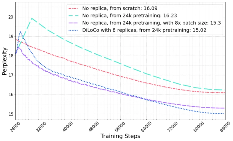
Figure 2 of Douillard et al. on DiLoCo (arXiv:2311.08105), reproduced for editorial coverage.

5A. The DiLoCo skeleton

Component: replicated local model. From the paper: Every worker $i$ holds a complete copy of $\theta$. [Analysis] This is the simplifying assumption that makes DiLoCo tractable to analyse; it also caps the model size at “what one worker can hold,” which OpenDiLoCo’s 1.1B-parameter run does not exceed. ^{1 2}

Component: AdamW inner optimizer. From the paper: Each worker runs $H$ AdamW steps locally with learning rate $\eta_{\text{inner}} = 4 \times 10^{-4}$ and weight decay 0.1. ¹ Plain English: each worker pretends, for the next $H$ steps, that it is training the model on its own. Design rationale: AdamW is the standard for transformer pre-training; using anything else would confound the comparison. What breaks if removed: replacing AdamW with SGD at the inner level destroys most of DiLoCo’s advantage. Classification: [Adopted], standard transformer-training practice.

Component: pseudo-gradient computation. From the paper: After $H$ inner steps, each worker computes its pseudo-gradient $\Delta_i^{(t)} = \theta^{(t-1)} - \theta_i^{(t)}$. ¹ Plain English: how far did each worker move from the global starting point? The pseudo-gradient is a parameter delta, not a true gradient, it has units of parameters, not of loss-per-parameter. Design rationale: the worker has done useful local optimisation work; the pseudo-gradient captures that work in a form the outer optimizer can consume. Classification: [Adopted], this is the FedAvg pattern. ⁴

Component: pseudo-gradient averaging via all-reduce. From the paper: $\bar{\Delta}^{(t)} = \frac{1}{k} \sum_{i=1}^{k} \Delta_i^{(t)}$, computed by an all-reduce-mean collective across workers. ¹ Plain English: each worker shares its pseudo-gradient with every other worker, and they all agree on the average. Design rationale: averaging reduces variance across the $k$ workers. Connection to pipeline: this is the one and only inter-worker communication event in DiLoCo, per outer step. Classification: [Adopted].

Component: outer SGD-with-Nesterov-momentum step. From the paper: The global model is updated as

$m^{(t)} = \beta m^{(t-1)} + \bar{\Delta}^{(t)}$

$\theta^{(t)} = \theta^{(t-1)} - \eta_{\text{outer}} (\beta m^{(t)} + \bar{\Delta}^{(t)})$

with $\eta_{\text{outer}} = 0.7$ and $\beta = 0.9$. ¹ Plain English: the outer step treats the averaged pseudo-gradient like a normal gradient and applies one Nesterov-momentum update with it. Design rationale: this is the load-bearing algorithmic choice, replacing the outer optimizer with plain SGD destroys most of the perplexity advantage; From the paper: ablations show AdamW + SGD outer is meaningfully worse than AdamW + Nesterov outer in both synchronous and asynchronous settings. ³ Classification: [New], prior FedAvg uses simple averaging (no momentum) at the outer step.

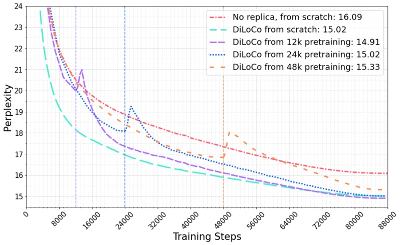
Figure 3 of Douillard et al. on DiLoCo (arXiv:2311.08105), reproduced for editorial coverage.

5B. OpenDiLoCo’s deployment-side changes

Component: Hivemind substrate. From the paper: OpenDiLoCo implements DiLoCo on top of the Hivemind library ⁹ using a distributed hash table for peer discovery and ring-allreduce for the outer step. ² Design rationale: NCCL-based all-reduce (the standard in single-cluster training) does not work across the open internet without a coordinator; Hivemind provides a peer-to-peer alternative that does. Classification: [Adapted]. Hivemind existed; OpenDiLoCo specialises it for the DiLoCo outer step.

Component: FP16 outer-step communication. From the paper: OpenDiLoCo all-reduces the pseudo-gradient in FP16 rather than FP32 and reports no perplexity degradation. ² Plain English: each parameter delta is transmitted in 16 bits instead of 32, halving the wire cost. Design rationale: the pseudo-gradient is, empirically, well-distributed enough that FP16 dynamic range is sufficient. What breaks if removed: nothing in terms of quality; the change is a pure efficiency win. Classification: [New].

Component: geographically-distributed deployment. From the paper: OpenDiLoCo demonstrates a run with four workers split across Canada, Finland, and the United States, with inter-worker bandwidth ranging from 127 to 935 Mbit/s, sustaining 90–95% compute utilization. ² Plain English: each worker keeps its GPUs busy for 90–95% of wall-clock time despite being on a different continent from the others. Classification: [New] at this scale; the algorithm allowed it, but no public paper had previously demonstrated it for LLM pre-training.

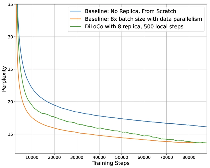
Figure 3 of Jaghouar, Ong, Hagemann on OpenDiLoCo (arXiv:2407.07852), reproduced for editorial coverage.

Figure 6 of Jaghouar, Ong, Hagemann on OpenDiLoCo (arXiv:2407.07852), reproduced for editorial coverage.

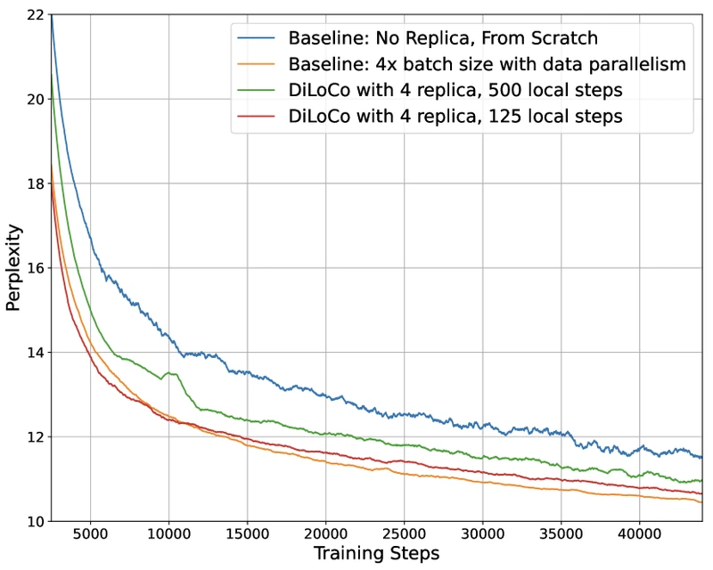
Figure 7 of Jaghouar, Ong, Hagemann on OpenDiLoCo (arXiv:2407.07852), reproduced for editorial coverage.

5C. AsyncDiLoCo’s algorithmic changes

Component: Delayed Nesterov (DN) outer optimizer. From the paper: Instead of applying Nesterov momentum on every outer step, DN accumulates pseudo-gradients in a buffer $\Delta_{\text{buf}}$ and applies the full Nesterov step only every $N_{\text{DN}}$ outer steps. Between Nesterov updates, the outer optimizer applies plain SGD with an optional small momentum fraction $c \in [0, 1/N_{\text{DN}}]$ (default $c = 0$). ³ Plain English: in async mode, the workers’ updates arrive one at a time at the server; if every arrival triggers a full Nesterov step, the momentum buffer ends up dominated by a single worker’s contribution rather than the average. DN batches updates first, then applies momentum. Classification: [New].

Component: Dynamic Local Updates (DyLU). From the paper: Worker $w$‘s local step count is set to $\lfloor v(w) / \max_{w'} v(w') \times H \rfloor$, where $v(w)$ is worker $w$‘s measured training speed in steps per second. ³ Plain English: the fastest worker runs $H$ local steps; slower workers run proportionally fewer, so all workers finish at roughly the same wall-clock time. Design rationale: this is a staleness-reduction trick, by aligning worker completion times, the server processes pseudo-gradients with similar effective staleness, which keeps the average meaningful. Classification: [New].

Component: progress-balanced data sharding. From the paper: Workers receive tasks with probability $p_i \propto \max(\mid D_i\mid /\sum_j \mid D_j\mid - n_i/\sum_j n_j, 0)$, where $n_i$ is the number of tokens worker $i$ has consumed so far. ³ Plain English: if a shard is behind on tokens consumed, future tasks are biased toward it. Design rationale: in heterogeneous settings, naive round-robin scheduling lets the fast workers race ahead on their shards while slow workers fall behind, creating an imbalanced training run. Classification: [New].

Component: grace-period synchronisation. From the paper: When a worker submits an update, the server waits a short grace period for additional workers to submit, batches them, and then immediately resumes if no more submissions arrive. ³ Plain English: a mini-batch of pseudo-gradients is processed together when convenient, but the server never blocks long. Classification: [New].

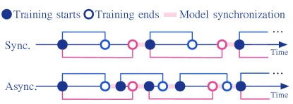
Figure 1 of Liu et al. on Asynchronous Local-SGD (arXiv:2401.09135), reproduced for editorial coverage.

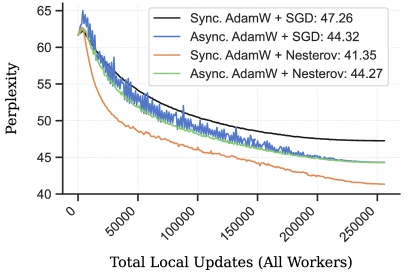
Figure 6 of Liu et al. on Asynchronous Local-SGD (arXiv:2401.09135), reproduced for editorial coverage.

Section 6: Mathematical contributions

MATH ENTRY 1: Pseudo-gradient

• Source: DiLoCo §3 / Algorithm 1 line “compute $\Delta_i$”. ¹
• What it is: the difference between the global model parameters at the start of an outer step and the worker’s local parameters at the end of $H$ inner steps. Plays the role of a gradient at the outer optimization level even though it is not the gradient of any single loss.
• Formal definition:

$\Delta_i^{(t)} = \theta^{(t-1)} - \theta_i^{(t)} \in \mathbb{R}^d$

• Each term explained and dimensional/type analysis.
  • $\theta^{(t-1)} \in \mathbb{R}^d$ is the global parameter vector at the start of outer step $t$.
  • $\theta_i^{(t)} \in \mathbb{R}^d$ is worker $i$‘s local parameter vector after $H$ AdamW steps starting from $\theta^{(t-1)}$.
  • $\Delta_i^{(t)} \in \mathbb{R}^d$ has the same shape as $\theta$ itself, it is a parameter delta, not a parameter scaled by a step size. Units: same as $\theta$.
• Worked numerical example. Let $d = 4$ (a 4-dimensional toy model) and $k = 2$ workers. Take $\theta^{(t-1)} = [1.0, 1.0, 1.0, 1.0]$. After 3 inner AdamW steps, worker 1 ends at $\theta_1^{(t)} = [0.96, 1.02, 0.94, 1.01]$ and worker 2 ends at $\theta_2^{(t)} = [0.94, 1.01, 0.97, 0.99]$. Then $\Delta_1^{(t)} = [0.04, -0.02, 0.06, -0.01]$ and $\Delta_2^{(t)} = [0.06, -0.01, 0.03, 0.01]$. The averaged pseudo-gradient is $\bar{\Delta}^{(t)} = [0.05, -0.015, 0.045, 0.0]$. Both workers descended on dimension 1 (positive $\Delta$ means $\theta$ decreased); they disagree on dimension 4, and the average cancels.
• Role. Input to the outer optimizer. Carries information about both the local data shard and the inner AdamW trajectory (which has its own preconditioning state).
• Edge cases. When $H = 1$, the pseudo-gradient collapses to $\eta_{\text{inner}}$ times the true (adaptively-preconditioned) gradient, and DiLoCo degenerates to standard data parallelism. When $H$ is very large, the pseudo-gradient may overshoot the global optimum for the worker’s local distribution, which is one source of the diminishing-returns ceiling.
• Novelty: [Adopted]. The pseudo-gradient idea is FedAvg-canonical. ⁴
• Transferability. [Analysis] Re-usable in any distributed-training context where workers are doing meaningful local optimisation; the formula does not depend on the inner optimizer being AdamW.
• Why it matters. It is the only object that crosses the network during DiLoCo training. Everything else stays local.

MATH ENTRY 2: DiLoCo outer Nesterov step

• Source: DiLoCo §3. ¹
• What it is: the rule by which the global model is updated using the averaged pseudo-gradient and a running momentum buffer.
• Formal definition:

$m^{(t)} = \beta m^{(t-1)} + \bar{\Delta}^{(t)}$

$\theta^{(t)} = \theta^{(t-1)} - \eta_{\text{outer}} \left( \beta m^{(t)} + \bar{\Delta}^{(t)} \right)$

• Each term explained and dimensional/type analysis.
  • $m^{(t)} \in \mathbb{R}^d$ is the Nesterov momentum buffer; same shape as $\theta$.
  • $\beta \in [0, 1)$ is the momentum coefficient (0.9 default). Dimensionless.
  • $\bar{\Delta}^{(t)} \in \mathbb{R}^d$ is the averaged pseudo-gradient from MATH ENTRY 1.
  • $\eta_{\text{outer}} \in \mathbb{R}_+$ is the outer learning rate (0.7 default). Dimensionless; multiplies the parameter-delta-shaped quantity to produce a parameter-delta-shaped update.
  • Note the Nesterov form: the update uses $\beta m^{(t)} + \bar{\Delta}^{(t)}$ rather than just $m^{(t)}$, which is the “look-ahead” term characteristic of Nesterov momentum.
• Worked numerical example. Continuing from MATH ENTRY 1, with $\bar{\Delta}^{(t)} = [0.05, -0.015, 0.045, 0.0]$, $m^{(t-1)} = [0.02, -0.01, 0.03, 0.005]$, $\beta = 0.9$, $\eta_{\text{outer}} = 0.7$:
  • $m^{(t)} = 0.9 \cdot [0.02, -0.01, 0.03, 0.005] + [0.05, -0.015, 0.045, 0.0] = [0.068, -0.024, 0.072, 0.0045]$.
  • Combined direction: $\beta m^{(t)} + \bar{\Delta}^{(t)} = [0.9 \cdot 0.068 + 0.05, \ldots] = [0.1112, -0.0366, 0.1098, 0.00405]$.
  • $\theta^{(t)} = [1.0, 1.0, 1.0, 1.0] - 0.7 \cdot [0.1112, -0.0366, 0.1098, 0.00405] = [0.9222, 1.0256, 0.9231, 0.9972]$.
  • Compare to a naive average update $\theta^{(t-1)} - \bar{\Delta}^{(t)} = [0.95, 1.015, 0.955, 1.0]$: the Nesterov step moves further on the high-confidence dimensions (1 and 3) where the momentum buffer already pointed the same way.
• Role. This is the global model’s update rule. It runs once per $H$ inner steps.
• Edge cases. If $\eta_{\text{outer}}$ is too large (say, $> 1.0$), the outer step overshoots and oscillates. If $\beta \approx 1$, the momentum buffer accumulates indefinitely; if $\beta = 0$, the outer optimizer degenerates to plain SGD on the pseudo-gradient.
• Novelty: [New]. Standard FedAvg has no outer momentum.
• Transferability. [Analysis] The exact $\eta_{\text{outer}} = 0.7, \beta = 0.9$ pairing is tuned for the C4 + transformer setting; recommended starting point on new domains is the same and then sweep $\eta_{\text{outer}} \in \{0.4, 0.7, 1.0\}$.
• Why it matters. It is the load-bearing algorithmic difference between DiLoCo and the prior local-SGD literature.

MATH ENTRY 3: Communication complexity per worker

• Source: DiLoCo §3 (implicit), OpenDiLoCo Table 2. ^{1 2}
• What it is: the number of bytes a single worker transmits to the rest of the cluster over a training run.
• Formal definition:

$\text{Comm}_{\text{DiLoCo}} = T \cdot 2 \cdot d \cdot b \cdot \frac{k-1}{k}$

versus

$\text{Comm}_{\text{DP}} = T \cdot H \cdot 2 \cdot d \cdot b \cdot \frac{k-1}{k}$

for ring-allreduce, where $b$ is bytes-per-parameter (4 for FP32, 2 for FP16) and the $\frac{k-1}{k}$ factor is the ring-allreduce bandwidth-optimal coefficient.

• Each term explained and dimensional/type analysis.
  • $T$: number of outer steps (dimensionless count).
  • $H$: inner steps per outer step (dimensionless count).
  • $d$: parameter count (e.g., $d = 1.5 \times 10^8$ for 150M model).
  • $b$: bytes-per-parameter; 4 for FP32, 2 for FP16.
  • $(k-1)/k$: bandwidth-optimal ring-allreduce coefficient; for $k=8$, this is 0.875.
• Worked numerical example. For a 150M-parameter model, $k = 8$, $H = 500$, $T = 88{,}000$ (DiLoCo’s main run):
  • DiLoCo FP16: $\text{Comm} = 88{,}000 \cdot 2 \cdot 1.5 \times 10^8 \cdot 2 \cdot 0.875 \approx 4.6 \times 10^{13}$ bytes $= 46$ TB per worker over the run.
  • Data-parallel FP16: $\text{Comm} \approx 23{,}100$ TB per worker, physically impossible across a residential link.
  • Ratio: $H = 500\times$ less communication, matching DiLoCo’s headline claim. ¹
• Role. This is the number that determines whether geographically-distributed training is feasible at all.
• Edge cases. If $k$ is very large, the $(k-1)/k$ factor approaches 1 and the algorithm becomes more bandwidth-bound; if $k = 2$, the ring degenerates to a single send-receive.
• Novelty: [Analysis] [Adopted], the formula is standard; the constant $H = 500$ is the contribution.
• Transferability. [Analysis] Re-usable for any communication-budget calculation in distributed training.
• Why it matters. It quantifies the headline 500× claim.

MATH ENTRY 4: Delayed Nesterov outer step (AsyncDiLoCo)

• Source: AsyncDiLoCo §4.2. ³
• What it is: the modified outer optimizer that asynchronously processes pseudo-gradients without letting Nesterov momentum amplify staleness.
• Formal definition (reconstructed from the paper’s description; the precise pseudocode is in the AsyncDiLoCo paper §4.2). Let $t$ index server-side update events (one per pseudo-gradient arrival). Let $\Delta_{\text{buf}}^{(t)}$ be the buffer:

$\Delta_{\text{buf}}^{(t)} = \Delta_{\text{buf}}^{(t-1)} + \tilde{\Delta}^{(t)}$

where $\tilde{\Delta}^{(t)}$ is the most recently submitted pseudo-gradient. The server applies:

$\theta^{(t)} = \theta^{(t-1)} - \eta_{\text{outer}} \cdot \tilde{\Delta}^{(t)} - c \cdot \eta_{\text{outer}} \cdot m^{(t-1)}$

between Nesterov updates (the “plain-SGD-with-small-momentum-fraction” branch with $c \in [0, 1/N_{\text{DN}}]$, default $c = 0$). When $(t+1) \bmod N_{\text{DN}} = 0$, the buffer flushes:

$m^{(t)} = \beta m^{(t-1)} + \Delta_{\text{buf}}^{(t)}$

$\theta^{(t)} = \theta^{(t-1)} - \eta_{\text{outer}} (\beta m^{(t)} + \Delta_{\text{buf}}^{(t)})$

$\Delta_{\text{buf}}^{(t)} \leftarrow 0$

• Each term explained.
  • $\tilde{\Delta}^{(t)}$ is one worker’s pseudo-gradient, not an average across workers (because workers submit asynchronously).
  • $\Delta_{\text{buf}}^{(t)}$ accumulates several workers’ pseudo-gradients before momentum is applied; same shape as $\theta$.
  • $N_{\text{DN}}$ is the buffer flush interval, typically $4$–$16$.
  • $c$: optional momentum fraction used between flushes; From the paper: default is $c = 0$. ³
• Worked numerical example. Suppose $N_{\text{DN}} = 4$, $\beta = 0.9$, $\eta_{\text{outer}} = 0.7$, $c = 0$, $d = 2$. Initial state $\theta = [1.0, 1.0]$, $m = [0, 0]$, $\Delta_{\text{buf}} = [0, 0]$. Worker A submits $\tilde{\Delta}^{(1)} = [0.04, -0.01]$. Between-flush branch: $\theta^{(1)} = [1.0 - 0.7 \cdot 0.04, 1.0 - 0.7 \cdot (-0.01)] = [0.972, 1.007]$. Buffer: $\Delta_{\text{buf}}^{(1)} = [0.04, -0.01]$. Worker B submits $\tilde{\Delta}^{(2)} = [0.03, 0.02]$: $\theta^{(2)} = [0.951, 0.993]$, $\Delta_{\text{buf}}^{(2)} = [0.07, 0.01]$. Worker C: $\tilde{\Delta}^{(3)} = [0.05, -0.005]$: $\theta^{(3)} = [0.916, 0.9965]$, $\Delta_{\text{buf}}^{(3)} = [0.12, 0.005]$. Worker D: $\tilde{\Delta}^{(4)} = [0.02, 0.01]$. Now $(t+1) \bmod 4 = 0$, so the flush branch fires: $\Delta_{\text{buf}}^{(4)} = [0.14, 0.015]$, $m^{(4)} = 0.9 \cdot [0, 0] + [0.14, 0.015] = [0.14, 0.015]$, $\theta^{(4)} = [0.916 - 0.7 \cdot (0.9 \cdot 0.14 + 0.14), 0.9965 - 0.7 \cdot (0.9 \cdot 0.015 + 0.015)] = [0.916 - 0.1862, 0.9965 - 0.01995] = [0.7298, 0.9766]$. Buffer resets to zero.
  • Compare to naive async (apply full Nesterov on every arrival): each of the 4 pseudo-gradients would have triggered a full momentum update, and the momentum buffer would have ended up dominated by the most-recent worker’s direction rather than the cluster average.
• Role. Replaces the synchronous DiLoCo outer optimizer when workers cannot synchronise on completion.
• Edge cases. If $N_{\text{DN}} = 1$, DN degenerates to naive async (one Nesterov step per arrival), which is the configuration the paper shows fails. If $N_{\text{DN}} = k$, DN approximates synchronous DiLoCo with a single accumulator.
• Novelty: [New]. The “delay the momentum” idea is the AsyncDiLoCo paper’s primary contribution.
• Transferability. [Analysis] Re-usable in any asynchronous training setup where momentum-staleness interaction is a concern; reportedly applies beyond LLMs.
• Why it matters. Without DN, async DiLoCo loses 1.5–3.0 perplexity points vs synchronous DiLoCo; with DN+DyLU, the gap is below 0.05 perplexity. ³

MATH ENTRY 5: Momentum amplification under naive async

• Source: AsyncDiLoCo §3.3. ³
• What it is: an explicit calculation showing why naive asynchronous application of Nesterov momentum to sequentially-arriving pseudo-gradients amplifies the apparent gradient magnitude.
• Formal derivation. Suppose $k = 4$ identical workers all submit the same pseudo-gradient $g$ in sequence, with the server applying a full Nesterov step per arrival. Starting from $m^{(0)} = 0$:
  • After arrival 1: $m^{(1)} = g$. Update: $-\eta(\beta g + g) = -\eta(1+\beta)g$.
  • After arrival 2: $m^{(2)} = \beta g + g = (1+\beta)g$. Update: $-\eta(\beta(1+\beta)g + g) = -\eta(1+\beta+\beta^2)g$.
  • After arrival 3: $m^{(3)} = \beta(1+\beta)g + g = (1+\beta+\beta^2)g$. Update coefficient: $-\eta(1 + \beta + \beta^2 + \beta^3)g$.
  • After arrival 4: $m^{(4)} = \beta^3 g + \beta^2 g + \beta g + g = \frac{1-\beta^4}{1-\beta}g$. Update coefficient: $-\eta(1+\beta)(1+\beta+\beta^2+\beta^3)g$ (the Nesterov look-ahead).
  • Total parameter change across the 4 arrivals. Summing the four updates gives the paper’s reported $-\eta(4 + 4\beta + 3\beta^2 + 2\beta^3 + \beta^4)g$ coefficient. For $\beta = 0.9$: $4 + 3.6 + 2.43 + 1.458 + 0.6561 \approx 12.14$, versus $4$ for plain SGD with the same gradients summed. ³ From the paper: “the momentum term becomes $\beta^4 m + (1 + \beta + \beta^2 + \beta^3) g$”, which is consistent with the per-arrival momentum recursion above. ³
• Intuition. Each pseudo-gradient triggers a full Nesterov step that compounds with the residual momentum from prior steps; with sequential application, the cluster’s effective learning rate is approximately $3\times$ what the synchronous-case calculation would predict.
• What this proves. The fix cannot be “reduce $\eta_{\text{outer}}$ by $3\times$” because the momentum buffer is also corrupted (it now reflects the most-recent worker’s direction, not the cluster average); the fix has to be structural (DN’s buffering).
• Worked numerical example. With $g = 1$, $\beta = 0.9$, $\eta = 0.7$: plain SGD update is $-2.8$ (four steps of $-0.7$); naive async Nesterov is approximately $-8.5$. The 3× ratio is what AsyncDiLoCo demonstrates as the failure mode.
• Role. Diagnostic; explains why DN exists.
• Novelty: [New]. The explicit per-arrival expansion is the AsyncDiLoCo paper’s diagnostic contribution.
• Why it matters. It is the only piece of pseudo-theory in the three papers; everything else is empirical.

MATH ENTRY 6: DyLU step-count rule

• Source: AsyncDiLoCo §4.3. ³
• What it is: the rule by which each worker’s local-step count is set proportional to its measured speed.
• Formal definition:

$H_w = \left\lfloor \frac{v(w)}{\max_{w' \in W} v(w')} \cdot H \right\rfloor$

• Each term explained. $v(w)$: worker $w$‘s training speed in steps per second. $H$: the fastest worker’s step budget per outer cycle. $H_w$: worker $w$‘s actual step count. $W$: the set of workers.
• Worked numerical example. Take 4 workers with measured speeds $v_1 = 100, v_2 = 80, v_3 = 60, v_4 = 50$ steps/second and $H = 500$. Then $H_1 = 500, H_2 = \lfloor 0.8 \cdot 500 \rfloor = 400, H_3 = 300, H_4 = 250$. All four finish their respective inner loops at the same wall-clock time: 5 seconds.
• Role. Aligns worker completion times to keep pseudo-gradient staleness uniform.
• Edge cases. If one worker is dramatically slower (say, $v < 0.1 \max v$), DyLU gives it almost no work, and the cluster effectively trains as $k - 1$ workers; in the limit of extreme heterogeneity, DyLU degenerates to “drop the slowest worker.”
• Novelty: [New].
• Transferability. [Analysis] Applicable to any synchronous distributed training where worker speeds vary at training time (cloud spot instances, mixed GPU generations).
• Why it matters. AsyncDiLoCo’s ablations show DyLU contributes about half of the wall-clock improvement over synchronous DiLoCo under heterogeneous-worker conditions. ³

Section 7: Algorithmic contributions

ALGORITHM ENTRY 1: DiLoCo (the headline algorithm)

• Source: DiLoCo Algorithm 1. ¹
• Purpose: Train one global LLM across $k$ workers with $H$ inner steps between synchronisations.
• Inputs: initial parameters $\theta^{(0)} \in \mathbb{R}^d$; data shards $D_1, \ldots, D_k$; inner optimizer (AdamW with $\eta_{\text{inner}}, \beta_1, \beta_2$, weight decay); outer optimizer (Nesterov with $\eta_{\text{outer}}, \beta$); outer steps $T$; inner steps per outer step $H$.
• Outputs: final global parameters $\theta^{(T)}$.

Headline algorithm rendered as PNG via image-fetch.mjs --mode code-block-image is embedded below; the inline reproduction:

Algorithm 1: DiLoCo
Input: theta_0, k workers, data shards D_1..D_k,
       InnerOpt = AdamW, OuterOpt = Nesterov
for outer step t = 1..T:
    for worker i = 1..k in parallel:
        theta_i = theta_{t-1}                       # broadcast global model
        for inner step h = 1..H:
            x ~ D_i                                  # sample local batch
            L = f(x, theta_i)                        # forward + loss
            theta_i = InnerOpt.step(theta_i, grad L) # AdamW update
        Delta_i = theta_{t-1} - theta_i              # pseudo-gradient
    Delta_bar = (1/k) * sum_i Delta_i                # all-reduce mean
    theta_t = OuterOpt.step(theta_{t-1}, Delta_bar)  # Nesterov outer update
return theta_T

• Hand-traced example on minimal input. Take $d = 2$ (toy two-parameter model), $k = 2$ workers, $H = 2$ inner steps, $T = 1$ outer step, $\theta^{(0)} = [1.0, 1.0]$.
  • Outer step $t = 1$:
    • Worker 1: $\theta_1 \leftarrow [1.0, 1.0]$. Inner step 1: sample $x_{1,1}$, compute gradient (toy values $[0.1, -0.05]$), AdamW step (assume effective step magnitude 0.01) yields $\theta_1 = [0.99, 1.005]$. Inner step 2: gradient $[0.08, -0.03]$, yields $\theta_1 = [0.982, 1.008]$. $\Delta_1 = [1.0, 1.0] - [0.982, 1.008] = [0.018, -0.008]$.
    • Worker 2: $\theta_2 \leftarrow [1.0, 1.0]$. Inner step 1: gradient $[0.06, -0.04]$, $\theta_2 = [0.994, 1.004]$. Inner step 2: gradient $[0.05, -0.03]$, $\theta_2 = [0.989, 1.007]$. $\Delta_2 = [0.011, -0.007]$.
    • Average: $\bar{\Delta} = [0.0145, -0.0075]$.
    • Outer step (with $m^{(0)} = [0, 0]$, $\beta = 0.9$, $\eta_{\text{outer}} = 0.7$): $m^{(1)} = [0.0145, -0.0075]$, $\theta^{(1)} = [1.0, 1.0] - 0.7 \cdot (0.9 \cdot [0.0145, -0.0075] + [0.0145, -0.0075]) = [1.0, 1.0] - 0.7 \cdot [0.02755, -0.01425] = [0.9807, 1.0100]$.
• Complexity. Time per outer step: $O(H \cdot \text{cost}(\text{forward+backward+AdamW}))$ for inner; $O(\text{all-reduce}(d))$ for outer. Space per worker: $O(d)$ for $\theta_i$ plus AdamW’s $2d$ moments plus outer optimizer’s $d$ momentum buffer. Total per worker: $\approx 4d$ parameter-equivalents. Communication per outer step: $O(d)$ one all-reduce.
• Bottleneck step explicitly named. The all-reduce at the outer step boundary. Inner steps run at full local speed.
• Hyperparameters.
  • $\eta_{\text{inner}} = 4 \times 10^{-4}$ (AdamW). From the paper: taken from standard LLM-pre-training practice; not aggressively tuned. ¹
  • $\eta_{\text{outer}} = 0.7$ (Nesterov). Sensitivity: AsyncDiLoCo’s ablations imply this is co-tuned with $\beta$ and is fragile. ³
  • $\beta = 0.9$ (Nesterov momentum). Standard.
  • $H = 500$. The headline value. Ablations show H=50 to H=1000 are all workable; H=500 is approximately the sweet spot. ¹
  • $k \in \{4, 8, 16, 64\}$ tested.
• Failure modes. Excessive $H$ (e.g., $H > 5000$) is reported as “diverges in non-i.i.d. settings” in DiLoCo §5. ¹ Excessive $\eta_{\text{outer}}$ overshoots. Mismatched inner/outer learning-rate scales corrupt the pseudo-gradient.
• Novelty: [New], the algorithm as a whole; component-wise [Adopted] for AdamW and all-reduce, [New] for the Nesterov outer optimizer choice in this setting.
• Transferability. [Analysis] Re-usable for any large-model pre-training where the cluster does not have NVLink-class interconnect; the recipe transfers as-is.

ALGORITHM ENTRY 2: OpenDiLoCo on Hivemind

• Source: OpenDiLoCo §2. ²
• Purpose: A peer-to-peer implementation of Algorithm 1 that does not require a central coordinator.
• Inputs: identical to Algorithm 1, plus a peer-discovery DHT bootstrap address and a peer-list refresh interval.
• Outputs: identical to Algorithm 1.
• Pseudocode.

Algorithm 2: OpenDiLoCo (Hivemind backend)
Input: theta_0, DHT bootstrap addrs, AdamW config, Nesterov config,
       fp16_grad_compress = True
on_each_worker:
    join_DHT()
    while not done:
        theta_local = pull_latest_global_theta()         # from DHT
        for inner step h = 1..H:
            x ~ local_data_shard
            L = f(x, theta_local)
            theta_local = AdamW.step(theta_local, grad L)
        Delta = theta_prev_global - theta_local
        Delta_fp16 = cast_to_fp16(Delta)                 # FP16 compression
        Delta_bar = hivemind_allreduce_mean(Delta_fp16)  # ring P2P all-reduce
        theta_global = Nesterov.step(theta_prev_global, Delta_bar)
        publish_global_theta_to_DHT(theta_global)

• Hand-traced example. Three workers in three different countries, each with a 150M model. Worker A (Canada, link 935 Mbit/s up to B, 127 Mbit/s up to C), Worker B (Finland), Worker C (USA). Each runs $H = 500$ AdamW steps on its local C4 shard for ~67.5 minutes (per the paper’s reported figure). ² Each casts its pseudo-gradient to FP16 (300 MB per worker for 150M parameters at 2 bytes/param). Hivemind ring-allreduce mean: total inter-worker traffic ≈ $2 \cdot 300 \cdot (3-1)/3 \approx 400$ MB per worker. At the slowest link (127 Mbit/s ≈ 16 MB/s), the all-reduce takes ~25 seconds; From the paper: all-reduce is ~6.9% of total training time. ² Each worker then applies the Nesterov outer step locally (identical because the all-reduce gives the same $\bar{\Delta}$ to everyone) and publishes the new global $\theta$ to the DHT.
• Complexity. Same as Algorithm 1, with FP16 halving the all-reduce wire cost.
• Hyperparameters. Same as Algorithm 1, plus Hivemind-specific DHT parameters (peer discovery interval, gossip timeout).
• Failure modes. Hivemind peer dropouts (a worker leaves mid-all-reduce) are handled by retrying the all-reduce with the remaining peers; [Analysis] this introduces a perplexity-level fairness question (the dropped worker’s pseudo-gradient is lost), but OpenDiLoCo does not quantify the effect.
• Novelty: [Adapted]. Hivemind existed; the FP16 outer-step compression is [New].
• Transferability. [Analysis] Directly re-usable. The Hivemind library is open-source.

ALGORITHM ENTRY 3: AsyncDiLoCo with DN + DyLU

• Source: AsyncDiLoCo Algorithm 1 (server) and Algorithm 2 (worker). ³
• Purpose: Remove the synchronous barrier so the cluster’s slowest worker does not bottleneck every outer step.
• Inputs: all of Algorithm 1, plus $N_{\text{DN}}$ (buffer flush interval), $c$ (between-flush momentum fraction, default 0), worker-speed estimates $v(w)$.
• Outputs: identical to Algorithm 1.
• Pseudocode (server side).

Algorithm 3a: AsyncDiLoCo Server
state: theta, m, Delta_buf, server_step_count t = 0
loop:
    grace_period_start = now()
    pending_workers = wait_for_one_submission()
    while now() - grace_period_start < grace_window:
        try:
            pending_workers += receive_more_submissions(timeout = 0)
        except timeout:
            break
    for tilde_Delta in pending_workers:
        t = t + 1
        if (t + 1) mod N_DN != 0:
            theta = theta - eta_outer * tilde_Delta - c * eta_outer * m
            Delta_buf = Delta_buf + tilde_Delta
        else:                                       # flush branch
            Delta_buf = Delta_buf + tilde_Delta
            m = beta * m + Delta_buf
            theta = theta - eta_outer * (beta * m + Delta_buf)
            Delta_buf = 0
    for worker in pending_workers:
        send_task(worker, theta, H_worker)          # next inner-loop assignment

• Pseudocode (worker side).

Algorithm 3b: AsyncDiLoCo Worker
on_task_receive(theta_global, H_w):
    theta_local = theta_global
    for inner step h = 1..H_w:                      # H_w = DyLU step count
        x ~ progress_balanced_sample(local_shard)
        L = f(x, theta_local)
        theta_local = AdamW.step(theta_local, grad L)
    submit(theta_global - theta_local)              # pseudo-gradient

• Hand-traced example on minimal input. Set $k = 3$ workers with $v = [100, 80, 50]$ steps/sec, $H = 100$, $N_{\text{DN}} = 3$, $\beta = 0.9$, $\eta_{\text{outer}} = 0.7$, $c = 0$. DyLU assigns $H_A = 100, H_B = 80, H_C = 50$. All three finish their inner loops at $t = 1$ second. Server receives three submissions within the grace window. Server step 1: $t = 1$, $(1+1) \bmod 3 = 2 \neq 0$, between-flush branch, $\theta \mathrel{-}= 0.7 \cdot \tilde{\Delta}_A$, $\Delta_{\text{buf}} = \tilde{\Delta}_A$. Server step 2: $t = 2$, $(2+1) \bmod 3 = 0$, flush! $\Delta_{\text{buf}} += \tilde{\Delta}_B$, $m = 0.9 \cdot 0 + \Delta_{\text{buf}} = \tilde{\Delta}_A + \tilde{\Delta}_B$, $\theta \mathrel{-}= 0.7 \cdot (0.9 \cdot m + \Delta_{\text{buf}})$, buffer resets. Server step 3: $t = 3$, $(3+1) \bmod 3 = 1$, between-flush, $\theta \mathrel{-}= 0.7 \cdot \tilde{\Delta}_C$, $\Delta_{\text{buf}} = \tilde{\Delta}_C$.
• Complexity. Same big-O as DiLoCo per outer step; the gain is in wall-clock idle reduction (15–25% per the paper’s measurements). ³
• Hyperparameters. $N_{\text{DN}}$ is the new tunable; From the paper: $N_{\text{DN}} \in \{4, 8, 16\}$ all work; default $N_{\text{DN}} = k$ (one flush per “round” of all workers). ³
• Failure modes. If $N_{\text{DN}} = 1$ (flush on every submission), DN degenerates to naive async and fails. If $N_{\text{DN}} \gg k$, the server applies plain SGD updates for too long between Nesterov steps and loses the momentum advantage.
• Novelty: [New], the algorithm is the AsyncDiLoCo paper’s primary contribution.
• Transferability. [Analysis] Re-usable in any asynchronous distributed training setup that combines an outer momentum optimizer with stochastic inner updates.

Section 8: Specialised design contributions

8A. LLM / prompt design

Not applicable to these papers. DiLoCo, OpenDiLoCo, and AsyncDiLoCo are pre-training methods; the prompts are next-token-prediction on C4. No prompt engineering.

8B. Architecture-specific details

From the paper: All three papers use a Chinchilla-style decoder-only transformer. DiLoCo tests three sizes: 60M (3 layers, hidden 896, 16 heads, K/V dim 64), 150M (12 layers, hidden 896, 16 heads, K/V dim 64), and 400M (12 layers, hidden 1536, 12 heads, K/V dim 128). ¹ OpenDiLoCo extends to 1.1B (Llama-architecture transformer). ² AsyncDiLoCo’s main experiments are at 20M, 60M, and 150M. ³ None of the three papers explores the algorithm at the 7B+ scale where current open-source pre-training releases sit; INTELLECT-1 (Prime Intellect) is the first 10B-class run. ¹⁰

8C. Training specifics

Hardware. DiLoCo: TPUv4 pods. OpenDiLoCo: A100 GPUs (single-node for ablations, geographically distributed for the headline run). AsyncDiLoCo: GPUs (specific generation not reported in the main text; the toy-code repo uses a single GPU). ¹¹

Batch size. Per-worker batch 512 sequences × 1024 tokens for DiLoCo’s main runs; ¹ OpenDiLoCo uses comparable configurations across model scales. ²

Steps / epochs. From the paper: DiLoCo’s main 150M run uses 88,000 outer steps × 500 inner steps each = 44M total optimizer steps. ¹

Warmup. [Reconstructed] Standard linear warmup of the inner-loop learning rate over the first few thousand inner steps; precise schedule not enumerated in the main text for all configurations. ¹

Gradient clipping. Not explicitly named in the DiLoCo paper’s main text; assumed at standard $\\mid \nabla\\mid _2 \leq 1.0$.

Mixed precision. DiLoCo: bf16 weights/activations with fp32 optimizer state. OpenDiLoCo: extends to FP16 on the outer all-reduce, which is the load-bearing efficiency contribution. ²

Data mixture. C4 (cleaned Common Crawl). Both i.i.d. and non-i.i.d. shardings are tested in DiLoCo; ¹ AsyncDiLoCo additionally tests four levels of worker-speed heterogeneity (none, slight, moderate, very) by artificially slowing some workers. ³

8D. Inference / deployment specifics

Not applicable. The trained model is a standard transformer; inference is unchanged.

Section 9: Experiments and results

Datasets. All three papers use C4 (Colossal Clean Crawled Corpus). DiLoCo also reports limited downstream-task numbers (LM eval harness). OpenDiLoCo focuses on language-modelling perplexity. AsyncDiLoCo focuses on perplexity and wall-clock time under heterogeneous workers.

Baselines.

• Single-worker training with batch size $k \times$ the per-worker batch (the “fair-compute” baseline).
• Synchronous data-parallel training with $k$ workers (the “communication-rich” baseline).
• For OpenDiLoCo additionally: PyTorch torch.distributed reference implementation of DiLoCo (the apples-to-apples comparison for the Hivemind variant).
• For AsyncDiLoCo additionally: naive async DiLoCo (no DN, no DyLU), Async + polynomial gradient downweighting, Async + delay-compensation, FedBuff-style buffering. ³

Evaluation metrics. Perplexity on C4 validation; wall-clock training time; compute utilization (MFU); communication volume (bytes per worker over the run); for AsyncDiLoCo, additional steady-state wall-clock improvement under heterogeneity.

Reproduced key result tables with attribution.

Table 1 — DiLoCo headline result on 8 workers (150M model, non-i.i.d. C4).

Configuration	Communication per outer step	Compute (×)	Perplexity
Baseline (1× batch, single worker)	0	1×	16.23
Baseline (8× batch, data-parallel)	$N$ all-reduces (one per inner step)	8×	15.30
DiLoCo (k=8, H=500)	$N/500$ all-reduces	8×	15.02

Source: DiLoCo Table 2, paraphrased. ¹ Table reproduced from DiLoCo (arXiv:2311.08105) for editorial coverage.

Table 2 — OpenDiLoCo headline result on 1.1B model.

Configuration	Workers	Local steps	Perplexity
Baseline (4× batch, data-parallel)	4	—	10.52
OpenDiLoCo (k=4, H=125)	4	125	10.76

Source: OpenDiLoCo §3. ² Reproduced for editorial coverage. The 0.24-point gap at 1.1B is the largest gap reported in any of the three papers, and OpenDiLoCo’s discussion attributes it to the smaller $H$ and the limited $T$ on the 1.1B run.

Table 3 — AsyncDiLoCo perplexity vs configuration on C4 (all values from AsyncDiLoCo’s main results table).

Configuration	20M	60M	150M
Synchronous DiLoCo	41.35	24.55	17.23
Naive Async DiLoCo	44.27	25.64	18.08
Async DN + DyLU (proposed)	41.13	24.53	17.26

Source: AsyncDiLoCo Table 1, paraphrased. ³ Reproduced for editorial coverage. The naive-async gap is 2.92 perplexity at 20M, 1.09 at 60M, 0.85 at 150M — the gap shrinks with scale but does not close, motivating DN+DyLU.

Main quantitative results.

• From the paper: DiLoCo: 8-worker DiLoCo at H=500 beats the 8× data-parallel baseline by ~0.28 perplexity at the 150M scale, with 500× less communication. ¹
• From the paper: OpenDiLoCo: 1.1B-parameter run with 4 workers achieves 10.76 perplexity vs 10.52 for 4× data-parallel, a 0.24 perplexity gap at 125× less communication. ²
• From the paper: AsyncDiLoCo: DN+DyLU matches synchronous DiLoCo per-update and beats it 15–25% in wall-clock time under heterogeneous workers. ³

Supplementary results. OpenDiLoCo’s geographically-distributed run sustained 90–95% MFU across Canada–Finland–USA with all-reduce consuming 6.9% of training time. ²

Ablations.

• Communication frequency $H$: DiLoCo tests $H \in \{50, 500, 1000\}$; H=500 is the sweet spot, H=1000 increases perplexity by 2.9% but reduces communication by another 2×. ¹
• Number of workers $k$: DiLoCo tests $k \in \{4, 8, 16, 64\}$; perplexity continues to improve up to $k = 64$ but the returns diminish past $k = 16$. ¹
• Outer optimizer: AsyncDiLoCo’s ablation shows AdamW + plain-SGD-outer is meaningfully worse than AdamW + Nesterov-outer in both sync and async modes. ³
• FP16 vs FP32 outer all-reduce (OpenDiLoCo): no measurable perplexity difference; the FP16 run halves outer-step bandwidth. ²
• Heterogeneity sweep (AsyncDiLoCo): at four levels of worker-speed variance, naive async DiLoCo is invariant (44.27 at 20M across all levels, the perplexity is dominated by the algorithmic problem, not the heterogeneity); DN+DyLU stays around 41.1 across all levels. ³

Hyperparameter sensitivity. The most sensitive hyperparameter is $\eta_{\text{outer}}$, co-tuned with $\beta$ and with the per-worker batch size; [Analysis] untested settings include very large $\beta$ ($> 0.95$), which would push the algorithm toward heavy-ball momentum behaviour. $N_{\text{DN}}$ (AsyncDiLoCo’s new tunable) is reportedly robust across $\{4, 8, 16\}$. ³

Robustness / stress tests. OpenDiLoCo’s geographically-distributed run is the most demanding stress test in the three papers; the algorithm sustains 90–95% utilization across asymmetric links and ~2,000 km of physical distance. ²

Qualitative results. None of the three papers report sample-level qualitative outputs from the trained models, the contribution is the training method, not the trained model. Prime Intellect’s INTELLECT-1 release later did publish samples from a 10B-scale OpenDiLoCo-trained model; ¹⁰ those are downstream of the three papers under review.

Experimental scope limits. [Analysis]

• No paper tests the algorithm at the 7B+ scale where current open-source pre-training sits. INTELLECT-1’s 10B run is the public empirical extension. ¹⁰
• No paper tests fine-tuning with DiLoCo (all are pre-training experiments).
• No paper tests mixture-of-experts models, where the per-worker memory footprint is sparse and the all-reduce volume is different.
• The geographically-distributed OpenDiLoCo run is a single-trajectory existence proof, not a statistical study; failure-mode characterisation (peer dropouts, link partitions, byzantine workers) is left to follow-up.

Independent benchmark cross-checks for SOTA claims. None of the three papers claims modelling SOTA; the claim is “matches synchronous data-parallel at $H$× less communication,” which is a property, not a benchmark ranking. [External comparison] Independent reproductions exist: Prime Intellect’s INTELLECT-1 ¹⁰ is an open-source 10B-parameter pre-training run on OpenDiLoCo across community-donated GPUs and serves as the largest external validation of the algorithm at the time of writing.

Evidence audit:

• Strongly supported: 500× communication reduction at 150M scale (DiLoCo); ¹ FP16 outer-step works (OpenDiLoCo); ² DN+DyLU closes the async-vs-sync gap (AsyncDiLoCo). ³
• Partially supported: 1.1B-scale claim has a 0.24 perplexity residual gap and is reported on a single run; ² the geographically-distributed run is one trajectory, not a distribution. ²
• Narrow evidence: behaviour at $k > 64$ workers; behaviour with peer dropouts; interaction with pipeline parallelism or MoE.

Section 10: Technical novelty summary

Component	Type	Novelty level	Justification	Source
Two-level inner-AdamW outer-Nesterov optimizer	Combination novel	Combines FedAvg’s local-steps idea with AdamW + Nesterov outer	DiLoCo §3 1
500× communication-frequency reduction at LLM scale	Fully novel	First demonstration at the LLM-pre-training scale	DiLoCo Table 2 1
FP16 outer all-reduce	Fully novel	First explicit demonstration that the pseudo-gradient tolerates FP16	OpenDiLoCo §3 2
Hivemind P2P implementation of DiLoCo	Combination novel	Hivemind existed; the DiLoCo-on-Hivemind integration is OpenDiLoCo’s contribution	OpenDiLoCo §2 2
Geographically-distributed LLM pre-training	Fully novel	First public demonstration sustaining 90–95% MFU across continents	OpenDiLoCo §4 2
Delayed Nesterov (DN) outer optimizer	Fully novel	The buffer-then-flush scheme has no direct precedent	AsyncDiLoCo §4.2 3
Dynamic Local Updates (DyLU)	Fully novel	Worker-speed-adaptive local step count	AsyncDiLoCo §4.3 3
Sequential-pseudo-gradient momentum amplification analysis	Fully novel	Diagnostic calculation explaining why naive async DiLoCo fails	AsyncDiLoCo §3.3 3

Single most novel contribution. [Analysis] DiLoCo’s most novel contribution is the empirical demonstration that AdamW + Nesterov-outer matches data-parallel quality at 500× less communication on a real LLM pre-training workload, the federated-learning algorithms had been around for years; the LLM-scale demonstration is what changed the systems-design conversation. OpenDiLoCo’s most novel contribution is the FP16-outer-all-reduce + Hivemind P2P substrate combination that makes the algorithm runnable on the open internet without a central coordinator. AsyncDiLoCo’s most novel contribution is the DN buffering scheme that converts an asynchrony failure mode into a workable algorithm.

What the papers do NOT claim to be novel. AdamW; Nesterov momentum (as an algorithm); FedAvg-style local steps; all-reduce; transformer architecture; C4; Hivemind (used as a library, not introduced); standard mixed-precision training.

Section 11: Situating the work

Prior work. Three direct intellectual ancestors. (1) FedAvg (McMahan et al., 2016) ⁴ introduced the local-steps + parameter-averaging pattern in the federated-learning setting, but used SGD as both inner and outer optimizer and did not scale to LLM pre-training. (2) Local SGD (Stich, 2018) ⁵ proved convergence guarantees for the local-then-average pattern in the convex case. (3) SlowMo (Wang et al., 2020) introduced the “post-local-step momentum” idea that DiLoCo’s outer Nesterov can be read as inheriting.

What this paper changes conceptually. Before DiLoCo, the systems literature treated cross-data-centre LLM training as infeasible, the per-step all-reduce volume was simply too high to traverse a multi-hop wide-area link. DiLoCo demonstrated that, at the LLM scale, the FedAvg trick was not just an option but a practical one with the right inner/outer optimizer combination. OpenDiLoCo turned this into an open-source artefact; AsyncDiLoCo removed the last “must finish at the same time” constraint. The architectural ceiling for who-can-train-frontier-LLMs moved from “who owns a hyperscale data centre” to “who can coordinate a cluster of nodes on the open internet.”

[External comparison] Contemporaneous related papers.

• DiLoCo Scaling Laws (Charles, Garrett, Reddi et al., 2025; arXiv:2503.09799) ⁶ . Extended scaling-law analysis of DiLoCo through 1B+ parameters showing that the algorithm’s compute-efficiency advantage grows with scale rather than shrinking. [Analysis] This is the strongest available extension of the DiLoCo claim at scale.
• Streaming DiLoCo with overlapping communication (Douillard et al., 2025; arXiv:2501.18512) ⁷ . Replaces the synchronous outer all-reduce with a streaming variant that overlaps with the inner computation, removing the all-reduce from the wall-clock critical path. [Analysis] This is the natural successor paper to OpenDiLoCo.
• Eager Updates (arXiv:2502.12996) ⁸ . A parallel line of work on overlapping communication and computation in DiLoCo; relates closely to Streaming DiLoCo but uses a different overlap discipline.

[Reviewer Perspective] Strongest skeptical objection. None of the three papers tests DiLoCo at the 7B+ scale where current open-source pre-training sits, and the largest published run in the three papers is OpenDiLoCo’s 1.1B model, a scale that fits comfortably in a single accelerator’s memory. The questions that arise above 7B (tensor-parallel-aware pseudo-gradients, pipeline-bubble interaction, optimizer-state-sharding compatibility) are not addressed; the algorithm has only been publicly validated above 7B by INTELLECT-1, ¹⁰ which is a community release rather than an academic paper with controlled baselines. Until a peer-reviewed paper validates DiLoCo at the 7B+ scale with proper baselines, the “this is the future of pre-training” framing is empirically under-supported.

[Reviewer Perspective] Strongest author-side rebuttal grounded in the paper. The DiLoCo line is a training-method paper, not a model-quality paper; the claim is that the algorithm preserves quality at a given compute budget while reducing communication. That claim is well-supported in the 60M–1.1B range tested, and there is no mechanistic reason the algorithm would fail at 7B beyond the engineering challenges of integrating it with tensor-parallel-sharded models. [Analysis] This rebuttal is procedurally sound but does not eliminate the empirical uncertainty.

What remains unsolved.

• Tensor-parallel compatibility: how does DiLoCo interact when each “worker” is itself a tensor-parallel cluster?
• Optimizer-state sharding: DiLoCo’s local AdamW state is per-worker; sharding it (à la ZeRO) is non-trivial in the DiLoCo framework.
• Heterogeneous-architecture clusters: the three papers assume identical-architecture workers; mixed-precision-capability clusters (some FP8, some FP16) are unstudied.
• Byzantine robustness: a malicious worker could submit a poisoned pseudo-gradient; the papers do not analyse this.

Three future research directions.

1. Pipeline-parallel-aware DiLoCo. When each worker is a multi-stage pipeline, the pseudo-gradient must be reconstructed coherently across stages. [Analysis] Likely a straightforward engineering problem with caveats around stage boundary conditions.
2. DiLoCo + MoE. Sparse-expert routing creates per-batch communication that does not respect the DiLoCo synchronisation boundary; the joint algorithm is open.
3. Theoretical convergence guarantees for DN. AsyncDiLoCo explicitly notes the lack of formal analysis; bridging the gap with Stich-style local-SGD theory is open.

Section 12: Critical analysis

Strengths with concrete evidence.

• DiLoCo’s 500× communication-frequency reduction is empirically validated against a fair-compute synchronous baseline at the 150M and 400M scales. ¹
• OpenDiLoCo’s open-source replication closes the “we believe DeepMind because they say so” gap that the original DiLoCo paper otherwise had; the 1.1B-parameter result is independently reproducible. ²
• AsyncDiLoCo’s DN+DyLU recipe converges to within 0.05 perplexity of synchronous DiLoCo across multiple model sizes and four heterogeneity levels. ³

Weaknesses explicitly stated by the authors.

• DiLoCo: “we have not investigated the role of the language modeling task itself”; the algorithm is plausibly task-dependent. ¹
• OpenDiLoCo: 1.1B-scale run is one trajectory; the 0.24 perplexity gap to data-parallel may shrink with longer training but is not closed in the paper. ²
• AsyncDiLoCo: “the precise cause of this issue remains unclear” regarding the momentum-staleness interaction at the theoretical level; ³ the Local-SGD advantage diminishes past 8 workers. ³

Weaknesses not stated or understated by the authors.

• [Reviewer Perspective] None of the three papers reports a failure trajectory. In a year of work, presumably some configurations diverged or stalled; reporting those would help practitioners avoid landmines. Independent commentary on the OpenDiLoCo replication notes that some hyperparameter combinations are fragile; ¹⁰ the academic papers do not.
• [Reviewer Perspective] The “500× less communication” headline elides that each outer all-reduce is still a full-parameter-vector traversal, which on 7B+ models is tens of GB. Practitioners pushing the algorithm to that scale care about latency per all-reduce, not just frequency.
• [Reviewer Perspective] AsyncDiLoCo’s DyLU assumes worker speeds are stable; on cloud spot-instance clusters, speeds can change minute-to-minute as neighbouring tenants contend for memory bandwidth. The paper’s heterogeneity sweep tests static speed assignments, not time-varying ones.

Reproducibility check.

• Code: DiLoCo: not released (DeepMind internal). OpenDiLoCo: open-source, MIT license. ² AsyncDiLoCo: toy example released, full code not released. ¹¹
• Data: C4 is public; data shards used are reproducible.
• Hyperparameters: DiLoCo: fully disclosed in §3. OpenDiLoCo: fully disclosed. AsyncDiLoCo: fully disclosed for the main runs; some ablation details (DN buffer size sweeps beyond the headline values) are partial.
• Compute: DiLoCo: reported as TPUv4 hours but exact node count not always reported per-experiment. OpenDiLoCo: reported. AsyncDiLoCo: not fully reported in the main text.
• Trained model weights: None of the three papers releases checkpoints. Prime Intellect’s INTELLECT-1 release does. ¹⁰
• Evaluation set: C4 validation, publicly reproducible.
• Overall: DiLoCo: partially reproducible (no code). OpenDiLoCo: fully reproducible. AsyncDiLoCo: partially reproducible.

Methodology disclosure.

Methodology (DiLoCo headline run):

• Sample size: $T \cdot H \cdot \text{batch} \approx 88{,}000 \cdot 500 \cdot 512 \approx 2.3 \times 10^{10}$ sequences per worker, $\times k = 8$ workers; 1024 tokens per sequence; $\approx 1.9 \times 10^{14}$ training tokens total.
• Evaluation set: C4 validation split.
• Baselines: single-worker 1× batch, 8-worker 8× batch data-parallel.
• Hardware / compute: TPUv4 pods; total compute budget not reported per-experiment in the main text.

Methodology (OpenDiLoCo 1.1B run):

• Sample size: not exhaustively reported; main run is $k=4, H=125$ for an undisclosed $T$.
• Evaluation set: C4 validation.
• Baselines: 4-worker 4× batch data-parallel.
• Hardware: A100 GPUs distributed across Canada, Finland, USA.

Methodology (AsyncDiLoCo main run):

• Sample size: standard 150M-scale C4 pre-training; exact step count not always reported per-ablation.
• Evaluation set: C4 validation.
• Baselines: synchronous DiLoCo, naive async, Async + Poly, Async + Delay Compensation, FedBuff-style Async Buffer.
• Hardware: not fully specified in the main text.

Generalisability.

• To larger scales: empirically open above 1.1B for the academic papers; INTELLECT-1 provides the 10B-scale data point. ¹⁰
• To other domains: the algorithm is data-modality-agnostic; the same Nesterov-outer choice should transfer to vision/multimodal pre-training, though no paper has demonstrated this.
• To fine-tuning: untested.
• To different backbones: tested across decoder-only transformers of different sizes; not tested on encoder-decoder or MoE.

Assumption audit. The strongest assumption is that each worker holds a full model copy; this caps DiLoCo at single-worker-memory-feasible models unless layered with tensor parallelism inside each worker. The second-strongest is that the data shards are similar enough in distribution that local AdamW state remains compatible across workers; the i.i.d.-vs-non-i.i.d. ablation in DiLoCo ¹ partially defends this but does not eliminate the concern at extreme non-i.i.d.

What would make the papers significantly stronger. [Analysis]

• A 7B-parameter, paper-quality experiment with controlled baselines.
• A formal convergence proof or at least a precise empirical characterisation of the regime where DN works.
• A taxonomy of failure modes (configurations that diverged, hyperparameters that destabilise), currently absent.

Section 13: What is reusable for a new study

REUSABLE COMPONENT 1: The DiLoCo two-level optimizer recipe

• What it is: AdamW inner + Nesterov outer, $H \approx 500$, $\eta_{\text{outer}} = 0.7$, $\beta = 0.9$.
• Why worth reusing: it is the only recipe with public empirical validation at the LLM pre-training scale.
• Preconditions: workers can each hold the full model; the inter-worker link can sustain one all-reduce per $H$ inner steps within a reasonable wall-clock fraction.
• What would need to change in a different setting: $H$ scales with the inter-worker link bandwidth (lower bandwidth → larger $H$); $\eta_{\text{outer}}$ is fragile and should be swept on new domains.
• Risks: the algorithm is sensitive to $\eta_{\text{outer}}$; mis-tuned outer rates either diverge or stall.
• Interaction effects: none with batch size beyond the standard data-parallel rules.

REUSABLE COMPONENT 2: FP16 outer all-reduce

• What it is: the pseudo-gradient is communicated in FP16, halving the wire cost.
• Why worth reusing: pure efficiency win at no perplexity cost in the OpenDiLoCo experiments. ²
• Preconditions: the all-reduce primitive supports FP16 (NCCL does; Hivemind does as of the OpenDiLoCo release).
• Risks: at much larger scales the FP16 dynamic range may not suffice; OpenDiLoCo does not test at 70B+.
• Interaction effects: none reported.

REUSABLE COMPONENT 3: Delayed Nesterov outer optimizer

• What it is: buffer $N_{\text{DN}}$ pseudo-gradients, apply Nesterov on flush, plain SGD between flushes.
• Why worth reusing: the only published recipe that makes asynchronous local-SGD work for the AdamW+Nesterov-outer combination.
• Preconditions: workers submit pseudo-gradients to a server (or peer set) at irregular intervals.
• What would need to change: $N_{\text{DN}}$ should be set close to $k$; the buffering policy needs to be aware of worker dropouts.
• Risks: if $N_{\text{DN}}$ is mis-set far from $k$, the algorithm either degenerates to naive async (too small) or loses the momentum advantage (too large).

REUSABLE COMPONENT 4: Dynamic Local Updates (DyLU)

• What it is: worker-speed-proportional local-step count.
• Why worth reusing: removes the straggler effect with one line of code; benefits any synchronous distributed training under speed heterogeneity.
• Preconditions: worker speeds are observable (or estimable) at training time.
• Risks: if worker speeds change mid-training, the assignment is stale; the paper’s heterogeneity sweep uses static speeds.

Dependency map. Component 1 (DiLoCo recipe) is the foundation. Components 2 (FP16 outer all-reduce) and 4 (DyLU) compose cleanly with 1. Component 3 (DN) replaces the outer optimizer in 1 and is mutually exclusive with the synchronous variant.

Recommendation. [Analysis] For a new study attempting decentralised LLM pre-training: start with Component 1 + Component 2 (synchronous DiLoCo with FP16 outer); add Component 4 (DyLU) when worker speeds are unequal; switch to Component 3 (DN) only when the synchronous barrier becomes the dominant wall-clock cost. This ordering matches OpenDiLoCo’s deployment progression.

[Analysis] What type of new study benefits most: a community-driven LLM training run on heterogeneous GPUs (the INTELLECT-1 use case) ¹⁰ is the canonical fit. Academic groups training on two co-located clusters with a shared 10 Gbps link will see smaller wins than residential-GPU pools.

Section 14: Known limitations and open problems

Limitations explicitly stated by the authors.

• DiLoCo: the algorithm is studied only in the language-modelling setting; transferability to other modalities is unstudied. ¹
• DiLoCo: behaviour at very large $H$ and very large $k$ is noted as future work. ¹
• OpenDiLoCo: the 1.1B run is a single trajectory; statistical replication is not reported. ²
• AsyncDiLoCo: the momentum-staleness interaction lacks a formal explanation; the Local-SGD advantage diminishes past 8 workers. ³

Limitations not stated.

• [Reviewer Perspective] No 7B-or-larger paper-quality experiment with proper baselines from any of the three papers; the gap is filled (informally) by INTELLECT-1’s community release rather than peer-reviewed work. ¹⁰
• [Reviewer Perspective] No characterisation of what happens when workers crash or partition. The Hivemind library handles it at the substrate level, but the algorithmic consequences are not analysed.
• [Analysis] The “communication per outer step” claim treats the outer all-reduce as a single event, but on multi-hop wide-area links the all-reduce latency dominates training when $H$ is moderate; a more honest cost metric would be “wall-clock fraction spent on all-reduce.” OpenDiLoCo reports this (6.9%) for one configuration but does not characterise it parametrically. ²

Technical root causes.

• Scale ceiling at 1.1B: limited by what each worker can hold; lifting it requires tensor-parallel-inside-each-worker support.
• Async-momentum staleness: root cause is the sequential-application amplification of Nesterov; DN addresses the symptom by batching.

Open problems.

• DiLoCo + MoE.
• DiLoCo + tensor parallelism within each worker.
• Byzantine-robust pseudo-gradient aggregation.
• Streaming / overlapped outer all-reduce (partially addressed by Streaming DiLoCo ⁷ and Eager Updates ⁸ , but not jointly with AsyncDiLoCo’s DN).
• Theoretical convergence proof for DN.

What a follow-up paper would need to solve to address the most critical limitation. [Analysis] The most critical limitation is the absence of a 7B+ paper-quality result. A follow-up would need to (a) integrate DiLoCo with tensor parallelism inside each worker, (b) demonstrate that the per-worker memory budget at 7B with TP=4 is workable, (c) run controlled baselines against a synchronous data-parallel 7B run on the same hardware, and (d) report the result with the same evaluation rigour as the 150M/400M papers. INTELLECT-1 ¹⁰ takes the first step toward (a)–(b) without (c)–(d).

How this article reads at three depths

For the curious high-school reader. Training a modern AI language model normally requires every GPU in a giant data centre to talk to every other GPU thousands of times per second. DiLoCo is a recipe that lets the GPUs talk to each other only every few minutes instead, each cluster trains the model on its own for a while, and then everyone averages the changes they made and continues from the average. OpenDiLoCo is the open-source version that scaled this idea up to billion-parameter models running across three countries. AsyncDiLoCo removes the rule that everyone has to finish at the same time, so slow GPUs no longer hold up the fast ones.

For the working developer or ML engineer. DiLoCo is FedAvg with two specific algorithmic choices that make it work for LLM pre-training: AdamW as the inner optimizer (matching standard practice) and Nesterov momentum as the outer optimizer applied to the averaged pseudo-gradient. The headline number is 500× fewer all-reduces at the 150M scale; at 1.1B the ratio drops to ~125× and the perplexity gap to data-parallel widens from negligible to about 0.24 points. OpenDiLoCo’s main practical contributions are the FP16 outer all-reduce (zero quality cost, halves wire bytes) and the Hivemind P2P backend (no central coordinator needed). When implementing: start synchronous, sweep $\eta_{\text{outer}}$ (the most fragile knob), then add FP16; only switch to AsyncDiLoCo’s DN+DyLU when worker stragglers dominate wall-clock time. The 7B+ regime is publicly demonstrated only by INTELLECT-1, not by the three academic papers.

For the ML researcher. The three papers establish a now-canonical recipe for decentralised LLM pre-training, with one load-bearing choice (Nesterov outer over plain SGD outer) and one load-bearing diagnostic (the sequential-pseudo-gradient momentum amplification calculation in AsyncDiLoCo §3.3) that motivates the DN buffering scheme. The strongest objection is the absence of a 7B+ paper-quality controlled experiment from any of the three papers; the strongest defence is that the algorithm is task-agnostic and the 60M–1.1B trajectory does not suggest scale-dependent failure. The most cite-worthy follow-up papers are the DiLoCo Scaling Laws (arXiv:2503.09799), Streaming DiLoCo (arXiv:2501.18512), and Eager Updates (arXiv:2502.12996), which together close the obvious gaps in the original three. A follow-up that integrates DiLoCo with tensor parallelism inside each worker and runs a controlled 7B baseline would, in this publication’s reading, complete the empirical story.